Make PICRUSt2 Output Analysis and Visualization Easier • ggpicrust2

ggpicrust2 is a comprehensive package that integrates pathway name/description annotations, ten of the most advanced differential abundance (DA) methods, and visualization of DA results. It offers a comprehensive solution for analyzing and interpreting the results of PICRUSt2 functional prediction in a seamless and intuitive way. Whether you are a researcher, data scientist, or bioinformatician, ggpicrust2 can help you better understand the underlying biological processes and mechanisms at play in your PICRUSt2 output data. So if you are interested in exploring the output data of PICRUSt2, ggpicrust2 is the tool you need.

Citation
Installation
Stay Updated
Workflow
Output
Function Details
FAQ
Author’s Other Projects

Citation

If you use ggpicrust2 in your research, please cite the following paper:

Chen Yang, Aaron Burberry, Xuan Cao, Jiahao Mai, Liangliang Zhang. (2023). ggpicrust2: an R package for PICRUSt2 predicted functional profile analysis and visualization. arXiv preprint arXiv:2303.10388.

BibTeX entry: @misc{yang2023ggpicrust2, title={ggpicrust2: an R package for PICRUSt2 predicted functional profile analysis and visualization}, author={Chen Yang and Aaron Burberry and Jiahao Mai and Xuan Cao and Liangliang Zhang}, year={2023}, eprint={2303.10388}, archivePrefix={arXiv}, primaryClass={stat.AP} }

ResearchGate preprint link: Click here

Installation

You can install the stable version of ggpicrust2 from CRAN with:

install.packages("ggpicrust2")

To install the latest development version of ggpicrust2 from GitHub, you can use:

# Install the devtools package if not already installed
# install.packages("devtools")

# Install ggpicrust2 from GitHub
devtools::install_github("cafferychen777/ggpicrust2")

Stay Updated

Follow me on Twitter for the latest ggpicrust2 updates:

Workflow

The easiest way to analyze the PICRUSt2 output is using ggpicrust2() function. The entire pipeline can be run with ggpicrust2() function.

ggpicrust2() integrates ko abundance to kegg pathway abundance conversion, annotation of pathway, differential abundance (DA) analysis, DA results visualization. When you have trouble running ggpicrust2(), you can debug it by running a separate function, which will greatly increase the speed of your analysis and visualization

ggpicrust2()

#If you want to analysis kegg pathway abundance instead of ko within the pathway. You should turn ko_to_kegg to TRUE.
#The kegg pathway typically have the more explainable description.
library(readr)
library(ggpicrust2)
library(tibble)
library(tidyverse)
library(ggprism)
library(patchwork)
metadata <-
  read_delim(
    "~/Microbiome/C9orf72/Code And Data/new_metadata.txt",
    delim = "\t",
    escape_double = FALSE,
    trim_ws = TRUE
  )
group <- "Enviroment"
daa_results_list <-
  ggpicrust2(
    file = "/Users/apple/Microbiome/C9orf72/Code And Data/picrust2_out/KO_metagenome_out/pred_metagenome_unstrat.tsv/pred_metagenome_unstrat.tsv",
    metadata = metadata,
    group = "Enviroment",
    pathway = "KO",
    daa_method = "LinDA",
    p_values_bar = TRUE,
    p.adjust = "BH",
    ko_to_kegg = TRUE,
    order = "pathway_class"
    select = NULL,
    reference = NULL # If your metadata[,group] has more than two levels, please specify a reference.
  )



#If you want to analysis the EC. MetaCyc. KO without conversions. You should turn ko_to_kegg to FALSE.
library(readr)
library(ggpicrust2)
library(tibble)
library(tidyverse)
library(ggprism)
library(patchwork)
metadata <-
  read_delim(
    "~/Microbiome/C9orf72/Code And Data/new_metadata.txt",
    delim = "\t",
    escape_double = FALSE,
    trim_ws = TRUE
  )
group <- "Enviroment"
daa_results_list <-
  ggpicrust2(
    file = "//Users/apple/Microbiome/C9orf72/Code And Data/picrust2_out/EC_metagenome_out/pred_metagenome_unstrat.tsv/pred_metagenome_unstrat.tsv",
    metadata = metadata,
    group = "Enviroment",
    pathway = "EC",
    daa_method = "LinDA",
    p_values_bar = TRUE,
    order = "group",
    ko_to_kegg = FALSE,
    x_lab = "description",
    p.adjust = "BH",
    select = NULL,
    reference = NULL
  )

If an error occurs with ggpicrust2, please use the following workflow.

#If you want to analysis kegg pathway abundance instead of ko within the pathway. You should turn ko_to_kegg to TRUE.
#The kegg pathway typically have the more explainable description.
#metadata should be tibble.
library(readr)
library(ggpicrust2)
library(tibble)
library(tidyverse)
library(ggprism)
library(patchwork)
metadata <-
  read_delim(
    "~/Microbiome/C9orf72/Code And Data/new_metadata.txt",
    delim = "\t",
    escape_double = FALSE,
    trim_ws = TRUE
  )

kegg_abundance <-
  ko2kegg_abundance(
    "/Users/apple/Downloads/pred_metagenome_unstrat.tsv/pred_metagenome_unstrat.tsv"
  )

group <- "Enviroment"

daa_results_df <-
  pathway_daa(
    abundance = kegg_abundance,
    metadata = metadata,
    group = group,
    daa_method = "ALDEx2",
    select = NULL,
    reference = NULL
  )

#if you are using LinDA, limme voom and Maaslin2, please specify a reference just like followings code.
# daa_results_df <- pathway_daa(abundance = kegg_abundance, metadata = metadata, group = group, daa_method = "LinDA", select = NULL, reference = "Harvard BRI")

daa_sub_method_results_df <-
  daa_results_df[daa_results_df$method == "ALDEx2_Kruskal-Wallace test", ]

daa_annotated_sub_method_results_df <-
  pathway_annotation(pathway = "KO",
                     daa_results_df = daa_sub_method_results_df,
                     ko_to_kegg = TRUE)

Group <-
  metadata$Enviroment # column which you are interested in metadata

# select parameter format in pathway_error() is c("ko00562", "ko00440", "ko04111", "ko05412", "ko00310", "ko04146", "ko00600", "ko04142", "ko00604", "ko04260", "ko04110", "ko04976", "ko05222", "ko05416", "ko00380", "ko05322", "ko00625", "ko00624", "ko00626", "ko00621")

daa_results_list <-
  pathway_errorbar(
    abundance = kegg_abundance,
    daa_results_df = daa_annotated_sub_method_results_df,
    Group = Group,
    p_values_threshold = 0.05,
    order = "pathway_class",
    select = NULL,
    ko_to_kegg = TRUE,
    p_value_bar = TRUE,
    colors = NULL,
    x_lab = "pathway_name"
  )
# x_lab can be set "feature" which represents kegg pathway id.

# If you want to analysis the EC. MetaCyc. KO without conversions. You should turn ko_to_kegg to FALSE.
library(readr)
library(ggpicrust2)
library(tibble)
library(tidyverse)
library(ggprism)
library(patchwork)
metadata <-
  read_delim(
    "~/Microbiome/C9orf72/Code And Data/new_metadata.txt",
    delim = "\t",
    escape_double = FALSE,
    trim_ws = TRUE
  )

#ko_abundance should be data.frame instead of tibble
#ID should be in the first column
ko_abundance <-
  read.delim(
    "/Users/apple/Downloads/pred_metagenome_unstrat.tsv/pred_metagenome_unstrat.tsv"
  )
#sometimes there are function, pathway or something else. Change function. when needed
rownames(ko_abundance) <- ko_abundance$function.
ko_abundance <- ko_abundance[, -1]

group <- "Enviroment"

daa_results_df <-
  pathway_daa(
    abundance = ko_abundance,
    metadata = metadata,
    group = group,
    daa_method = "ALDEx2",
    select = NULL,
    reference = NULL
  )

#if you are using LinDA, limme voom and Maaslin2, please specify a reference just like followings code.
# daa_results_df <- pathway_daa(abundance = kegg_abundance, metadata = metadata, group = group, daa_method = "LinDA", select = NULL, reference = "Harvard BRI")

daa_sub_method_results_df <-
  daa_results_df[daa_results_df$method == "ALDEx2_Kruskal-Wallace test", ]

daa_annotated_sub_method_results_df <-
  pathway_annotation(pathway = "KO",
                     daa_results_df = daa_sub_method_results_df,
                     ko_to_kegg = FALSE)

Group <-
  metadata$Enviroment # column which you are interested in metadata

# select parameter format in pathway_error() is c("K00001", "K00002", "K00003", "K00004")

daa_results_list <-
  pathway_errorbar(
    abundance = ko_abundance,
    daa_results_df = daa_annotated_sub_method_results_df,
    Group = Group,
    p_values_threshold = 0.05,
    order = "pathway_class",
    select = NULL,
    ko_to_kegg = FALSE,
    p_value_bar = TRUE,
    colors = NULL,
    x_lab = "description"
  )

Output

The typical output of the ggpicrust2 is like this.

function details

ko2kegg_abundance()

KEGG Orthology(KO) is a classification system developed by the Kyoto Encyclopedia of Genes and Genomes (KEGG) data-base(Kanehisa et al., 2022). It uses a hierarchical structure to classify enzymes based on the reactions they catalyze. To better understand pathways’ role in different groups and classify the pathways, the KO abundance table needs to be converted to KEGG pathway abundance. But PICRUSt2 removes the function from PICRUSt. ko2kegg_abundance() can help convert the table.

# Sample usage of the ko2kegg_abundance function

# Assume that the KO abundance table is stored in a file named "ko_abundance.tsv"

ko_abundance_file <- "ko_abundance.tsv"

kegg_abundance <- ko2kegg_abundance(ko_abundance_file)

# The resulting kegg_abundance data frame can now be used for further analysis and visualization.

pathway_daa()

Differential abundance(DA) analysis plays a major role in PICRUSt2 downstream analysis. pathway_daa() integrates almost all DA methods applicable to the predicted functional profile which there excludes ANCOM and ANCOMBC. It includes ALDEx2(Fernandes et al., 2013), DEseq2(Love et al., 2014), Maaslin2(Mallick et al., 2021), LinDA(Zhou et al., 2022), edgeR(Robinson et al., 2010) , limma voom(Ritchie et al., 2015), metagenomeSeq(Paulson et al., 2013), lefser(Segata et al., 2011).

#the abundance table is better to be data.frame rather than tibble
#you can use ko2_kegg_abundance output
abundance <- ko2kegg_abundance(ko_abundance_file)
metadata <-
  read_delim(
    "~/Microbiome/C9orf72/Code And Data/new_metadata.txt",
    delim = "\t",
    escape_double = FALSE,
    trim_ws = TRUE
  )
group <- "Enviroment"
#daa_method default is "ALDex2"
daa_results_df <- pathway_daa(abundance = abundance,
           metadata = metadata,
           group = group ,
           daa_method = "limma voom",
           select = NULL,
           p.adjust = "BH",
           reference = NULL)
#If you group levels >3 and want to use the LinDA, limme voom and Maaslin2, you should give a reference.
metadata <-
  read_delim(
    "~/Microbiome/C9orf72/Code And Data/new_metadata.txt",
    delim = "\t",
    escape_double = FALSE,
    trim_ws = TRUE
  )
group <- "Group"
daa_results_df <- pathway_daa(abundance = abundance,
           metadata = metadata,
           group = group ,
           daa_method = "limma voom",
           select = NULL,
           p.adjust = "BH",
           reference = "Harvard BRI")

pathway_annotation()

If you are in China and you are using kegg pathway annotation, Please make sure your internet can break through the firewall.

daa_results_df <- pathway_annotation(pathway = "KO", daa_results_df = daa_results_df, ko_to_kegg = TRUE)

pathway_errorbar()

pathway_errorbar(abundance = abundance,
           daa_results_df = daa_results_df,
           Group = metadata$Enviroment,
           ko_to_kegg = TRUE,
           p_values_threshold = 0.05,
           order = "pathway_class",
           select = NULL,
           p_value_bar = TRUE,
           colors = NULL,
           x_lab = NULL)

pathway_heatmap()

In this section, we will demonstrate how to create a pathway heatmap using the pathway_heatmap function in the ggpicrust2 package. This function visualizes the relative abundance of pathways in different samples.

First, we will create some example functional pathway abundance data and metadata:

# Create example functional pathway abundance data
abundance_example <- matrix(rnorm(30), nrow = 10, ncol = 3)
rownames(abundance_example) <- paste0("Sample", 1:10)
colnames(abundance_example) <- c("PathwayA", "PathwayB", "PathwayC")

# Create example metadata
# Please change your sample id's column name to sample_name
metadata_example <- data.frame(sample_name = rownames(abundance_example),
                               group = factor(rep(c("Control", "Treatment"), each = 5)))

Next, we will use the pathway_heatmap function to create a heatmap:

# Create a heatmap
heatmap_plot <- ggpicrust2::pathway_heatmap(t(abundance_example), metadata_example, "group")

Finally, we will display the resulting heatmap:

print(heatmap_plot)

pathway_pca()

In this section, we will demonstrate how to perform Principal Component Analysis (PCA) on functional pathway abundance data and create visualizations of the PCA results using the pathway_pca function in the ggpicrust2 package.

First, we will create some example functional pathway abundance data and metadata:

# Create example functional pathway abundance data
abundance_example <- data.frame(A = rnorm(10), B = rnorm(10), C = rnorm(10))

# Create example metadata
metadata_example <- tibble::tibble(sample_id = 1:10,
                                   group = factor(rep(c("Control", "Treatment"), each = 5)))

Next, we will use the pathway_pca function to perform PCA and create visualizations:

# Perform PCA and create visualizations
pca_plot <- ggpicrust2::pathway_pca(t(abundance_example), metadata_example, "group")

Finally, we will display the resulting PCA plot:

print(pca_plot)

FAQ

Issue 1: pathway_errorbar error

When using pathway_errorbar with the following parameters:

pathway_errorbar(abundance = abundance,
                 daa_results_df = daa_results_df,
                 Group = metadata$Enviroment,
                 ko_to_kegg = TRUE,
                 p_values_threshold = 0.05,
                 order = "pathway_class",
                 select = NULL,
                 p_value_bar = TRUE,
                 colors = NULL,
                 x_lab = "pathway_name")

You may encounter an error:

Error in `ggplot_add()`:
! Can't add `e2` to a <ggplot> object.
Run `rlang::last_trace()` to see where the error occurred.

Make sure you have the patchwork package loaded:

library(patchwork)

Issue 2: guide_train.prism_offset_minor error

You may encounter an error with guide_train.prism_offset_minor:

Error in guide_train.prism_offset_minor(guide, panel_params[[aesthetic]]) : 
  No minor breaks exist, guide_prism_offset_minor needs minor breaks to work

Ensure that the ggprism package is loaded:

library(ggprism)

Issue 3: SSL certificate problem

When encountering the following error:

SSL peer certificate or SSH remote key was not OK: [rest.kegg.jp] SSL certificate problem: certificate has expired

If you are in China, make sure your computer network can bypass the firewall.

Issue 4: Bad Request (HTTP 400)

When encountering the following error:

Error in .getUrl(url, .flatFileParser) : Bad Request (HTTP 400).

Please restart R session.

Issue 5: Error in grid.Call(C_textBounds, as.graphicsAnnot(xlabel),xx, xy, :

When encountering the following error:

Error in grid.Call(C_textBounds, as.graphicsAnnot(xlabel),x$x, x$y, :

Please having some required fonts installed. You can refer to this thread.

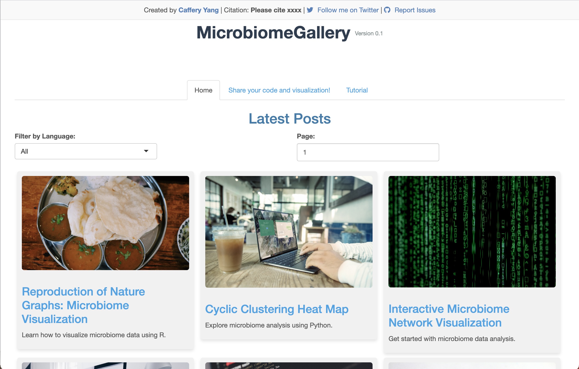
Author’s other projects

MicrobiomeGallery, a web-based platform for sharing microbiome data visualization code and datasets. （It’s still under construction）

ggpicrust2 Documentation

Table of Contents

Citation

Installation

Stay Updated

Workflow

ggpicrust2()

If an error occurs with ggpicrust2, please use the following workflow.

Output

function details

ko2kegg_abundance()

pathway_daa()

pathway_annotation()

pathway_errorbar()

pathway_heatmap()

pathway_pca()

FAQ

Issue 1: pathway_errorbar error

Issue 2: guide_train.prism_offset_minor error

Issue 3: SSL certificate problem

Issue 4: Bad Request (HTTP 400)

Issue 5: Error in grid.Call(C_textBounds, as.graphicsAnnot(xlabel),xx, xy, :

Author’s other projects

ggpicrust2 Documentation

Table of Contents

Citation

Installation

Stay Updated

Workflow

ggpicrust2()

If an error occurs with ggpicrust2, please use the following workflow.

Output

function details

ko2kegg_abundance()

pathway_daa()

pathway_annotation()

pathway_errorbar()

pathway_heatmap()

pathway_pca()

Share

FAQ

Issue 1: pathway_errorbar error

Issue 2: guide_train.prism_offset_minor error

Issue 3: SSL certificate problem

Issue 4: Bad Request (HTTP 400)

Issue 5: Error in grid.Call(C_textBounds, as.graphicsAnnot(xlabel),xx, xy, :

Author’s other projects