
Generates various plots to visualize relative abundance of taxa or functions for both cross-sectional and longitudinal microbiome data.
Usage
plot_feature_diversity(
  data.obj,
  group.var = NULL,
  strata.var = NULL,
  subject.var = NULL,
  time.var = NULL,
  time.point.plot,
  is.plot.change = TRUE,
  feature.change.func = "relative change",
  feature.level = NULL,
  feature.dat.type = c("count", "proportion", "other"),
  features.plot = NULL,
  prop.to.lump = 1e-04,
  top.k.plot = NULL,
  top.k.func = NULL,
  plot.other = TRUE,
  renormalize = FALSE,
  plot.scheme = c("combined", "individual"),
  plot.type = c("barplot", "dotplot", "areaplot", "heatmap", "spaghettiplot", "boxplot",
    "scatterplot")
)
Arguments
- data.obj
A MicrobiomeStat data object, which is a list containing at minimum the following components:
feature.tab: A matrix of feature abundances (taxa/genes as rows, samples as columns)meta.dat: A data frame of sample metadata (samples as rows)
Optional components include:
feature.ann: A matrix/data frame of feature annotations (e.g., taxonomy)tree: A phylogenetic tree object (class "phylo")feature.agg.list: Pre-aggregated feature tables by taxonomy
Data objects can be created using converters like
mStat_convert_phyloseq_to_data_objor importers likemStat_import_qiime2_as_data_obj.- group.var
Character string specifying the column name in meta.dat containing the grouping variable (e.g., treatment, condition, phenotype). Used for between-group comparisons.
- strata.var
Character string specifying the column name in meta.dat for stratification. When provided, analyses and visualizations will be performed separately within each stratum (e.g., by site, batch, or sex).
- subject.var
Character string specifying the column name in meta.dat that uniquely identifies each subject or sample unit. Required for longitudinal and paired designs to track repeated measurements.
- time.var
Character string specifying the column name in meta.dat containing the time variable. Required for longitudinal and paired analyses. Supports character/factor labels (e.g., "baseline", "week4") and numeric values. Some trend/volatility methods require numeric or coercible-to-numeric time values.
- time.point.plot
Character vector of time points to plot.
- is.plot.change
Logical, plot change from baseline (only for multiple time points).
- feature.change.func
Method for calculating change: "relative change", "log fold change", or "absolute change".
- feature.level
Character vector specifying the taxonomic or annotation level(s) for analysis. Should match column names in feature.ann, such as "Phylum", "Family", "Genus", etc. Use "original" to analyze at the original feature level without aggregation.
- feature.dat.type
Character string specifying the data type of feature.tab. One of:
"count": Raw count data (will be normalized)
"proportion": Relative abundance data (should sum to 1 per sample)
"other": Pre-transformed data (no transformation applied)
- features.plot
Character vector of specific feature IDs to plot (default NULL plots all).
- prop.to.lump
Numeric, features below this mean proportion are lumped into "other".
- top.k.plot
Integer, number of top features to plot.
- top.k.func
Function to rank features for top.k selection.
- plot.other
Logical, whether to include "other" category in plots.
- renormalize
Logical, renormalize after removing "other" category.
- plot.scheme
Character, "combined" or "individual" plot layout.
- plot.type
Character, plot type: "barplot", "dotplot", "areaplot", "heatmap", "spaghettiplot", "boxplot", or "scatterplot".
Examples
# \donttest{
data(ecam.obj)
plot_feature_diversity(
data.obj = ecam.obj,
group.var = "antiexposedall",
strata.var = NULL,
time.var = "month",
time.point.plot = unique(ecam.obj$meta.dat$month)[1],
is.plot.change = TRUE,
feature.level = c("Phylum", "Family", "Genus"),
feature.dat.type = "proportion",
features.plot = NULL,
prop.to.lump = 0.0001,
top.k.plot = NULL,
top.k.func = NULL,
renormalize = FALSE,
plot.other = TRUE,
plot.scheme = "combined",
plot.type = "barplot"
)
#> Validation passed.
#> Validation passed.
#> Data has been subsetted based on the provided samIDs.
#> Updated metadata to match the subsetted data.
#> 801 samples were excluded.
#> Updated feature table to match the subsetted data.
#> Feature annotation remains aligned to the current feature set.
#> Data subsetting complete. Returning updated data object.
#> Your data is in proportion format. For barplot visualization, additional normalization is not required as ggplot2's position='fill' will automatically handle the proportions.
#> Warning: No shared levels found between `names(values)` of the manual scale and the
#> data's colour values.
#> Warning: No shared levels found between `names(values)` of the manual scale and the
#> data's colour values.
#> Validation passed.
#> Validation passed.
#> Data has been subsetted based on the provided samIDs.
#> Updated metadata to match the subsetted data.
#> 801 samples were excluded.
#> Updated feature table to match the subsetted data.
#> Feature annotation remains aligned to the current feature set.
#> Data subsetting complete. Returning updated data object.
#> Your data is in proportion format. For barplot visualization, additional normalization is not required as ggplot2's position='fill' will automatically handle the proportions.
#> Warning: No shared levels found between `names(values)` of the manual scale and the
#> data's colour values.
#> Warning: No shared levels found between `names(values)` of the manual scale and the
#> data's colour values.
#> Validation passed.
#> Validation passed.
#> Data has been subsetted based on the provided samIDs.
#> Updated metadata to match the subsetted data.
#> 801 samples were excluded.
#> Updated feature table to match the subsetted data.
#> Feature annotation remains aligned to the current feature set.
#> Data subsetting complete. Returning updated data object.
#> Your data is in proportion format. For barplot visualization, additional normalization is not required as ggplot2's position='fill' will automatically handle the proportions.
#> Warning: No shared levels found between `names(values)` of the manual scale and the
#> data's colour values.
#> Warning: No shared levels found between `names(values)` of the manual scale and the
#> data's colour values.
#> $Phylum
#> $Phylum$Phylum
#> $Phylum$Phylum$indiv
#> Warning: No shared levels found between `names(values)` of the manual scale and the
#> data's colour values.
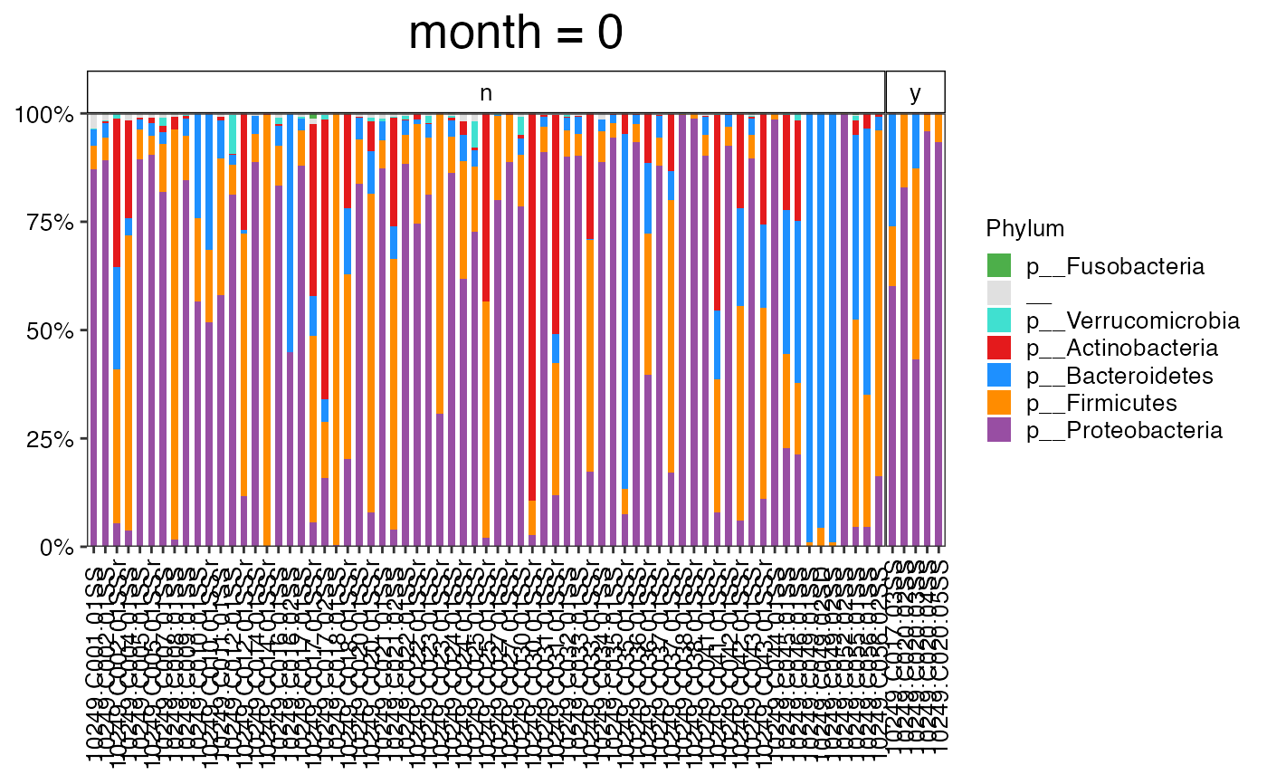 #>
#> $Phylum$Phylum$average
#> Warning: No shared levels found between `names(values)` of the manual scale and the
#> data's colour values.
#>
#> $Phylum$Phylum$average
#> Warning: No shared levels found between `names(values)` of the manual scale and the
#> data's colour values.
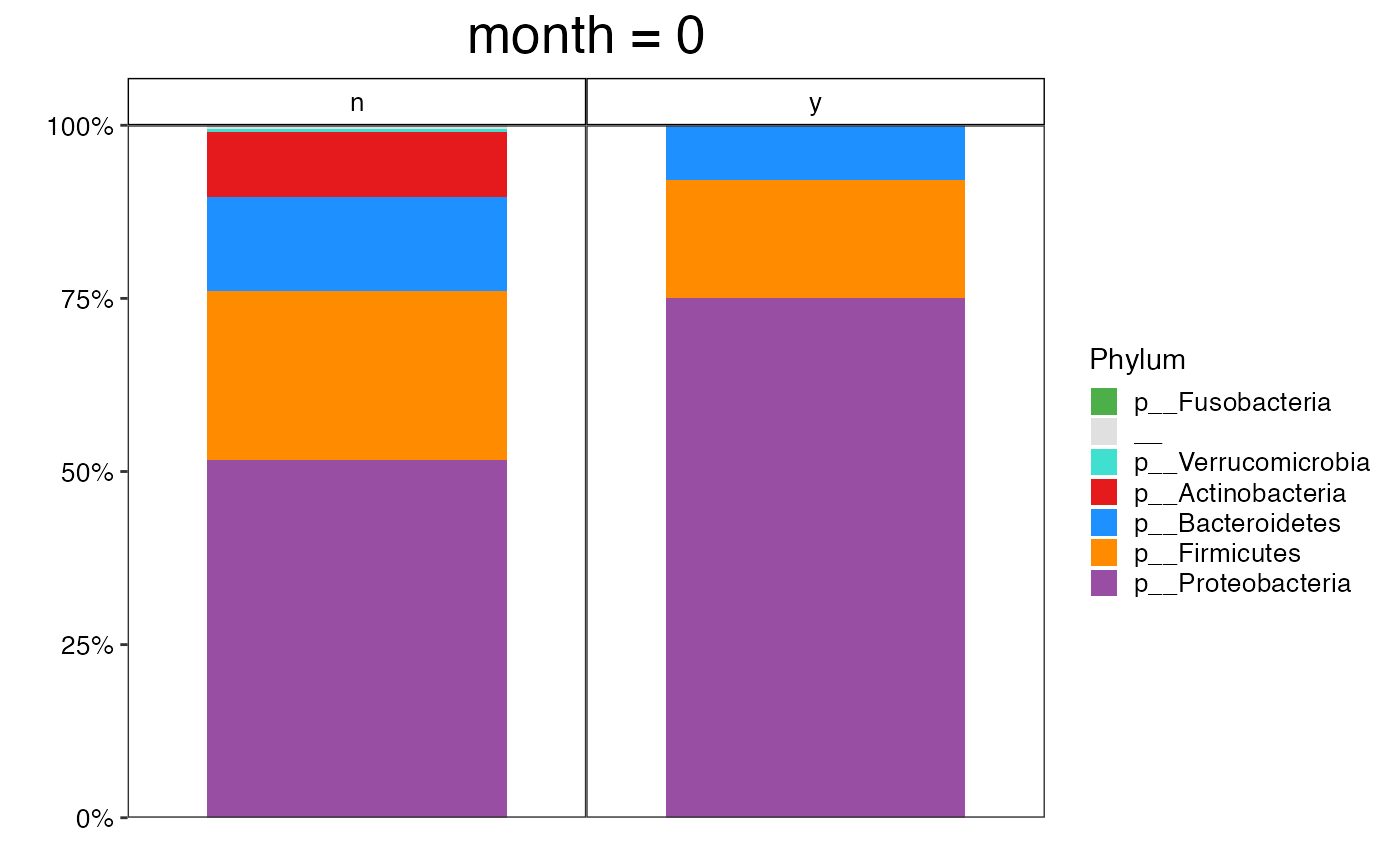 #>
#>
#>
#> $Family
#> $Family$Family
#> $Family$Family$indiv
#> Warning: No shared levels found between `names(values)` of the manual scale and the
#> data's colour values.
#>
#>
#>
#> $Family
#> $Family$Family
#> $Family$Family$indiv
#> Warning: No shared levels found between `names(values)` of the manual scale and the
#> data's colour values.
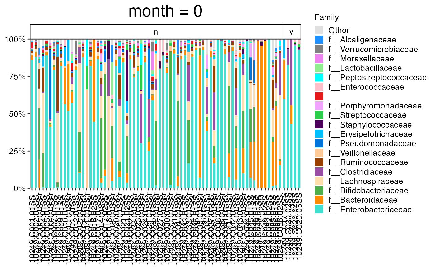 #>
#> $Family$Family$average
#> Warning: No shared levels found between `names(values)` of the manual scale and the
#> data's colour values.
#>
#> $Family$Family$average
#> Warning: No shared levels found between `names(values)` of the manual scale and the
#> data's colour values.
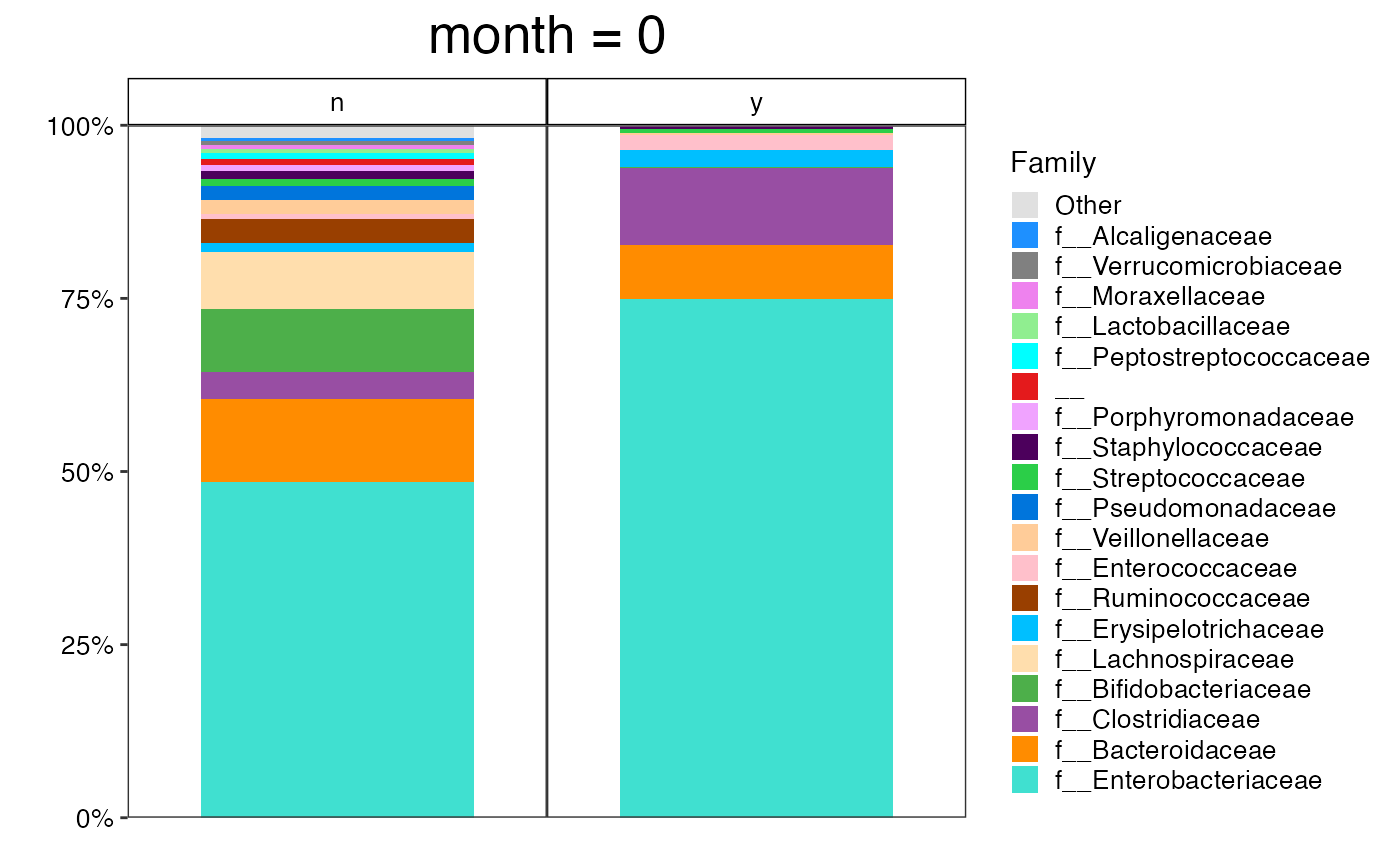 #>
#>
#>
#> $Genus
#> $Genus$Genus
#> $Genus$Genus$indiv
#> Warning: No shared levels found between `names(values)` of the manual scale and the
#> data's colour values.
#>
#>
#>
#> $Genus
#> $Genus$Genus
#> $Genus$Genus$indiv
#> Warning: No shared levels found between `names(values)` of the manual scale and the
#> data's colour values.
 #>
#> $Genus$Genus$average
#> Warning: No shared levels found between `names(values)` of the manual scale and the
#> data's colour values.
#>
#> $Genus$Genus$average
#> Warning: No shared levels found between `names(values)` of the manual scale and the
#> data's colour values.
 #>
#>
#>
plot_feature_diversity(
data.obj = ecam.obj,
group.var = "antiexposedall",
strata.var = "delivery",
time.var = "month",
time.point.plot = unique(ecam.obj$meta.dat$month)[1],
is.plot.change = TRUE,
feature.level = c("Phylum", "Family", "Genus"),
feature.dat.type = "proportion",
features.plot = NULL,
prop.to.lump = 0.0001,
top.k.plot = NULL,
top.k.func = NULL,
renormalize = FALSE,
plot.other = TRUE,
plot.scheme = "combined",
plot.type = "barplot"
)
#> Validation passed.
#> Validation passed.
#> Data has been subsetted based on the provided samIDs.
#> Updated metadata to match the subsetted data.
#> 801 samples were excluded.
#> Updated feature table to match the subsetted data.
#> Feature annotation remains aligned to the current feature set.
#> Data subsetting complete. Returning updated data object.
#> Your data is in proportion format. For barplot visualization, additional normalization is not required as ggplot2's position='fill' will automatically handle the proportions.
#> Warning: No shared levels found between `names(values)` of the manual scale and the
#> data's colour values.
#> Warning: No shared levels found between `names(values)` of the manual scale and the
#> data's colour values.
#> Validation passed.
#> Validation passed.
#> Data has been subsetted based on the provided samIDs.
#> Updated metadata to match the subsetted data.
#> 801 samples were excluded.
#> Updated feature table to match the subsetted data.
#> Feature annotation remains aligned to the current feature set.
#> Data subsetting complete. Returning updated data object.
#> Your data is in proportion format. For barplot visualization, additional normalization is not required as ggplot2's position='fill' will automatically handle the proportions.
#> Warning: No shared levels found between `names(values)` of the manual scale and the
#> data's colour values.
#> Warning: No shared levels found between `names(values)` of the manual scale and the
#> data's colour values.
#> Validation passed.
#> Validation passed.
#> Data has been subsetted based on the provided samIDs.
#> Updated metadata to match the subsetted data.
#> 801 samples were excluded.
#> Updated feature table to match the subsetted data.
#> Feature annotation remains aligned to the current feature set.
#> Data subsetting complete. Returning updated data object.
#> Your data is in proportion format. For barplot visualization, additional normalization is not required as ggplot2's position='fill' will automatically handle the proportions.
#> Warning: No shared levels found between `names(values)` of the manual scale and the
#> data's colour values.
#> Warning: No shared levels found between `names(values)` of the manual scale and the
#> data's colour values.
#> $Phylum
#> $Phylum$Phylum
#> $Phylum$Phylum$indiv
#> Warning: No shared levels found between `names(values)` of the manual scale and the
#> data's colour values.
#>
#>
#>
plot_feature_diversity(
data.obj = ecam.obj,
group.var = "antiexposedall",
strata.var = "delivery",
time.var = "month",
time.point.plot = unique(ecam.obj$meta.dat$month)[1],
is.plot.change = TRUE,
feature.level = c("Phylum", "Family", "Genus"),
feature.dat.type = "proportion",
features.plot = NULL,
prop.to.lump = 0.0001,
top.k.plot = NULL,
top.k.func = NULL,
renormalize = FALSE,
plot.other = TRUE,
plot.scheme = "combined",
plot.type = "barplot"
)
#> Validation passed.
#> Validation passed.
#> Data has been subsetted based on the provided samIDs.
#> Updated metadata to match the subsetted data.
#> 801 samples were excluded.
#> Updated feature table to match the subsetted data.
#> Feature annotation remains aligned to the current feature set.
#> Data subsetting complete. Returning updated data object.
#> Your data is in proportion format. For barplot visualization, additional normalization is not required as ggplot2's position='fill' will automatically handle the proportions.
#> Warning: No shared levels found between `names(values)` of the manual scale and the
#> data's colour values.
#> Warning: No shared levels found between `names(values)` of the manual scale and the
#> data's colour values.
#> Validation passed.
#> Validation passed.
#> Data has been subsetted based on the provided samIDs.
#> Updated metadata to match the subsetted data.
#> 801 samples were excluded.
#> Updated feature table to match the subsetted data.
#> Feature annotation remains aligned to the current feature set.
#> Data subsetting complete. Returning updated data object.
#> Your data is in proportion format. For barplot visualization, additional normalization is not required as ggplot2's position='fill' will automatically handle the proportions.
#> Warning: No shared levels found between `names(values)` of the manual scale and the
#> data's colour values.
#> Warning: No shared levels found between `names(values)` of the manual scale and the
#> data's colour values.
#> Validation passed.
#> Validation passed.
#> Data has been subsetted based on the provided samIDs.
#> Updated metadata to match the subsetted data.
#> 801 samples were excluded.
#> Updated feature table to match the subsetted data.
#> Feature annotation remains aligned to the current feature set.
#> Data subsetting complete. Returning updated data object.
#> Your data is in proportion format. For barplot visualization, additional normalization is not required as ggplot2's position='fill' will automatically handle the proportions.
#> Warning: No shared levels found between `names(values)` of the manual scale and the
#> data's colour values.
#> Warning: No shared levels found between `names(values)` of the manual scale and the
#> data's colour values.
#> $Phylum
#> $Phylum$Phylum
#> $Phylum$Phylum$indiv
#> Warning: No shared levels found between `names(values)` of the manual scale and the
#> data's colour values.
 #>
#> $Phylum$Phylum$average
#> Warning: No shared levels found between `names(values)` of the manual scale and the
#> data's colour values.
#>
#> $Phylum$Phylum$average
#> Warning: No shared levels found between `names(values)` of the manual scale and the
#> data's colour values.
 #>
#>
#>
#> $Family
#> $Family$Family
#> $Family$Family$indiv
#> Warning: No shared levels found between `names(values)` of the manual scale and the
#> data's colour values.
#>
#>
#>
#> $Family
#> $Family$Family
#> $Family$Family$indiv
#> Warning: No shared levels found between `names(values)` of the manual scale and the
#> data's colour values.
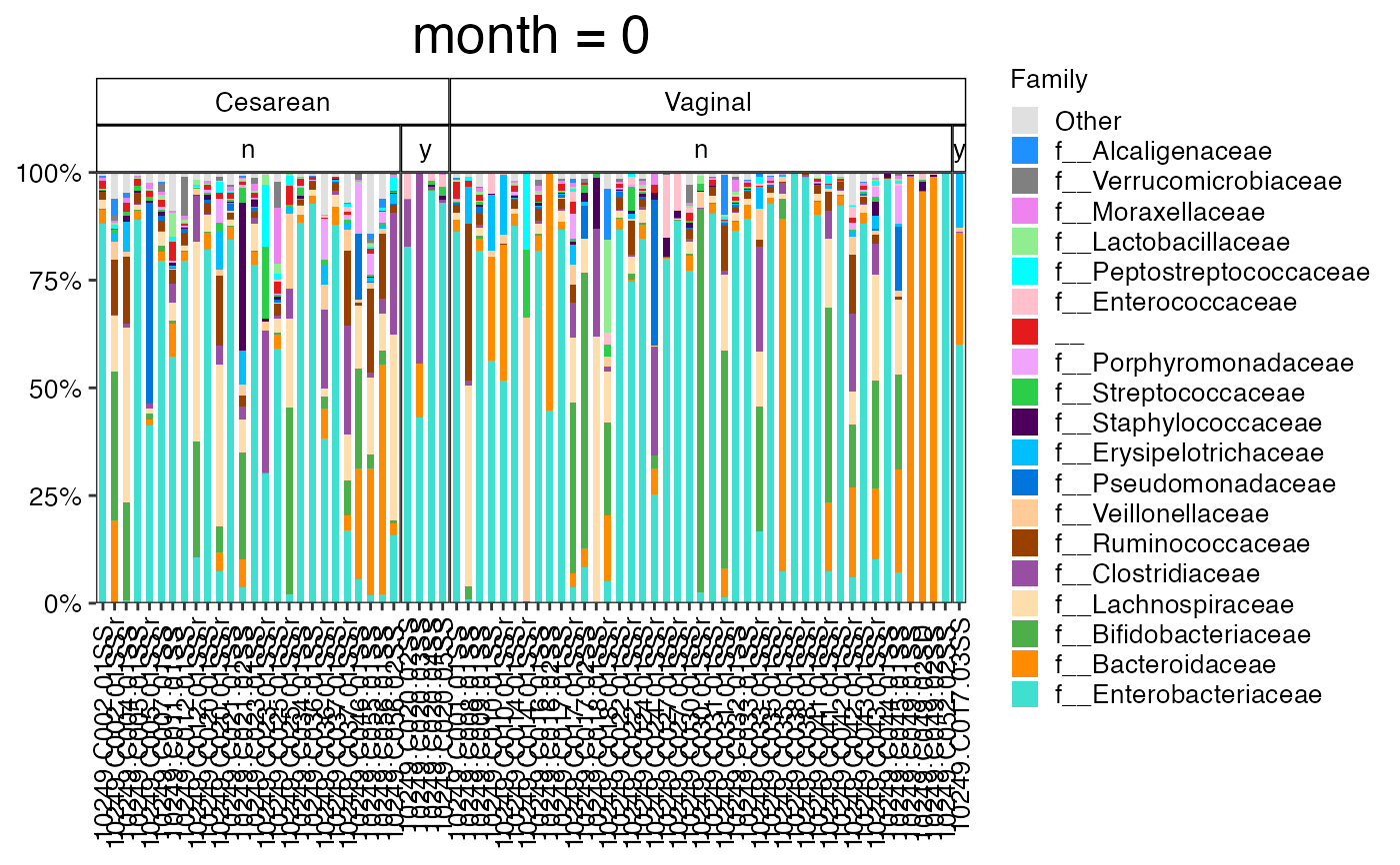 #>
#> $Family$Family$average
#> Warning: No shared levels found between `names(values)` of the manual scale and the
#> data's colour values.
#>
#> $Family$Family$average
#> Warning: No shared levels found between `names(values)` of the manual scale and the
#> data's colour values.
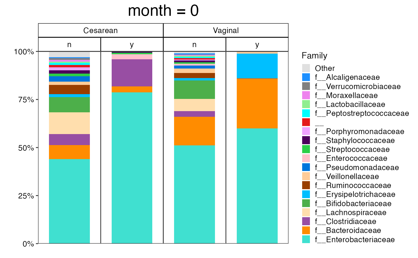 #>
#>
#>
#> $Genus
#> $Genus$Genus
#> $Genus$Genus$indiv
#> Warning: No shared levels found between `names(values)` of the manual scale and the
#> data's colour values.
#>
#>
#>
#> $Genus
#> $Genus$Genus
#> $Genus$Genus$indiv
#> Warning: No shared levels found between `names(values)` of the manual scale and the
#> data's colour values.
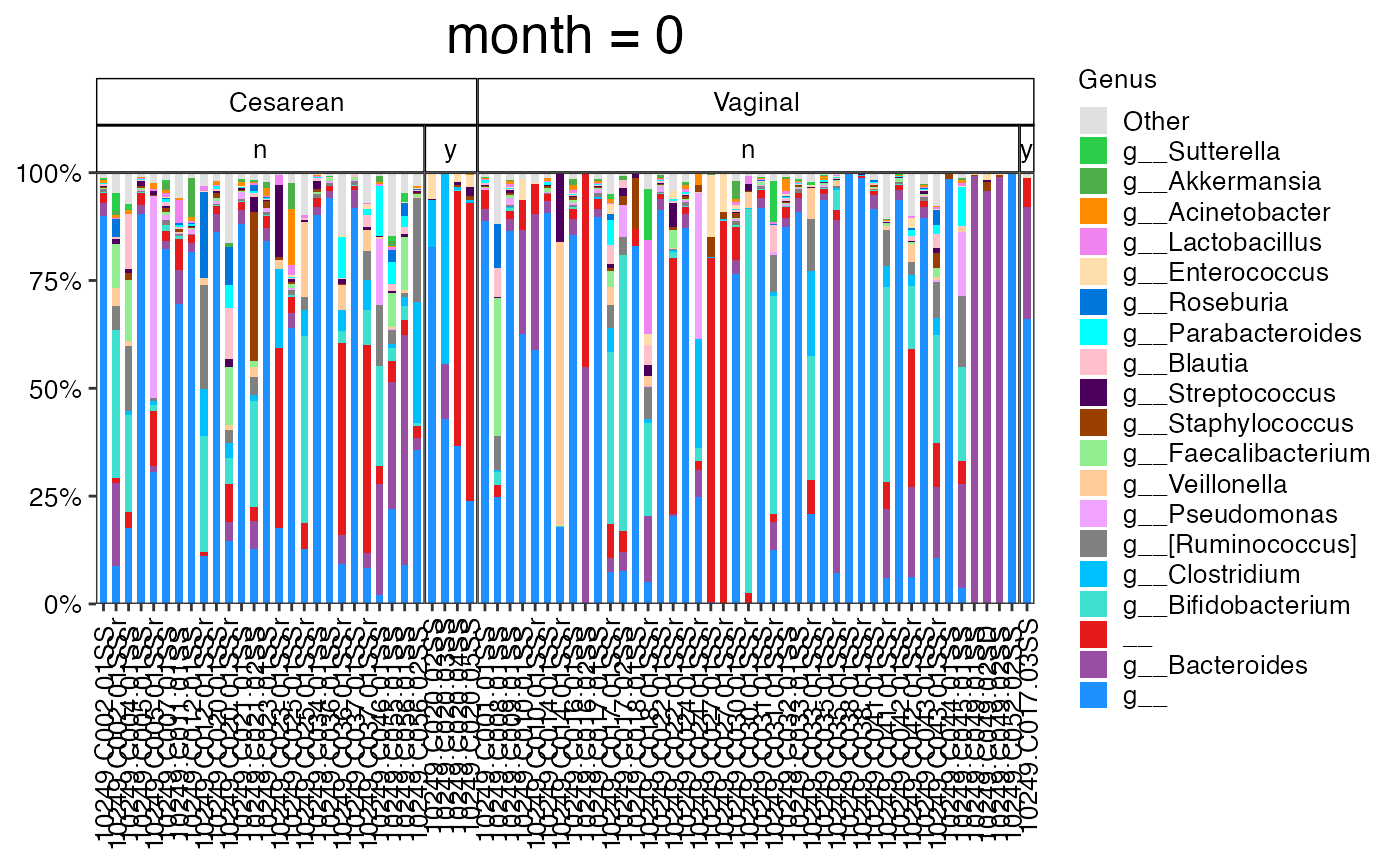 #>
#> $Genus$Genus$average
#> Warning: No shared levels found between `names(values)` of the manual scale and the
#> data's colour values.
#>
#> $Genus$Genus$average
#> Warning: No shared levels found between `names(values)` of the manual scale and the
#> data's colour values.
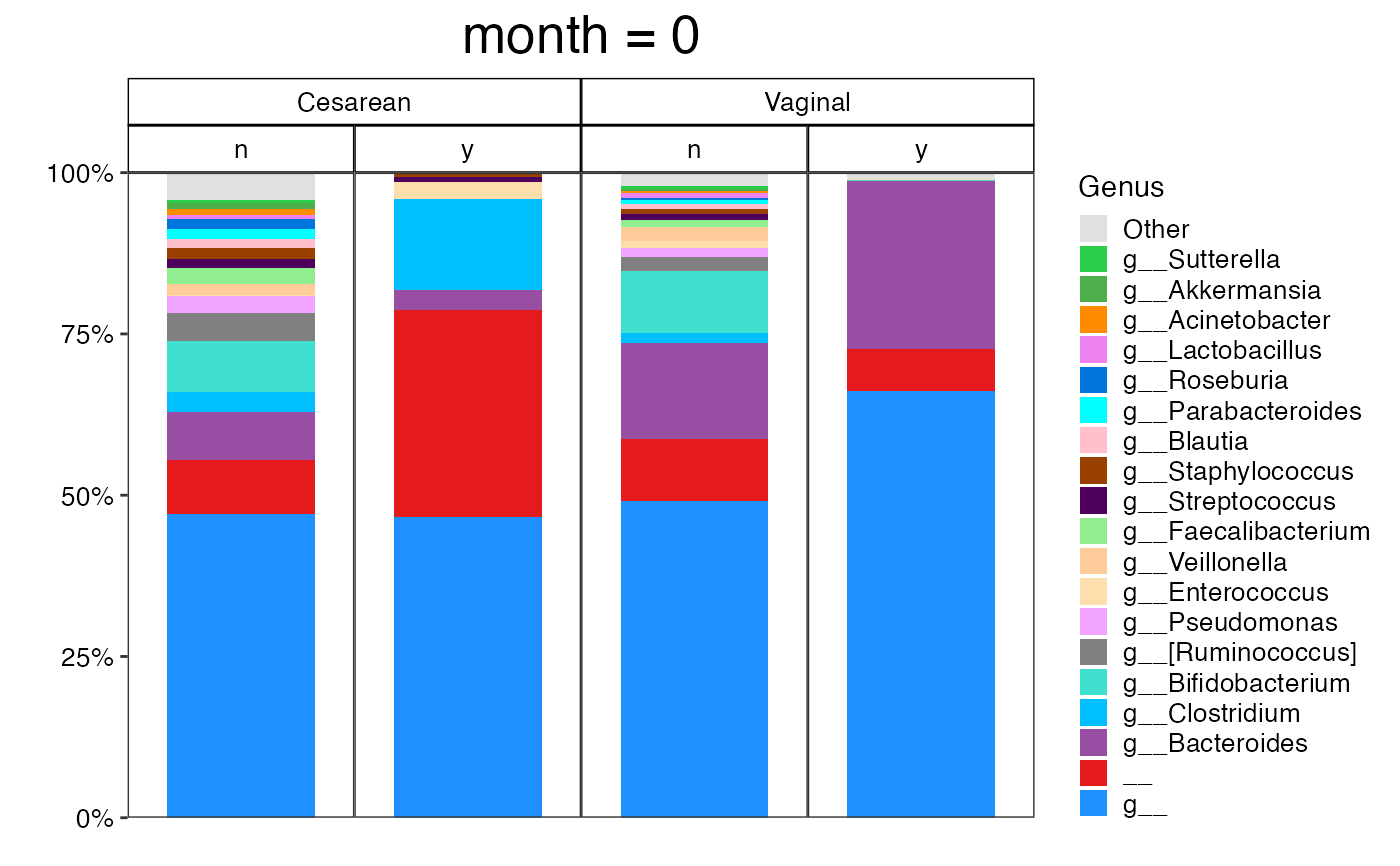 #>
#>
#>
# Get valid Phylum values (excluding empty strings and NAs)
valid_phyla <- unique(ecam.obj$feature.ann[,"Phylum"])
valid_phyla <- valid_phyla[!valid_phyla %in% c("__", "") & !is.na(valid_phyla)]
plot_feature_diversity(
data.obj = ecam.obj,
group.var = "antiexposedall",
strata.var = "delivery",
time.var = "month",
time.point.plot = unique(ecam.obj$meta.dat$month)[1],
is.plot.change = TRUE,
feature.level = c("Phylum"),
feature.dat.type = "proportion",
features.plot = valid_phyla[1:3],
prop.to.lump = 0.0001,
top.k.plot = NULL,
top.k.func = NULL,
renormalize = FALSE,
plot.other = TRUE,
plot.scheme = "combined",
plot.type = "barplot"
)
#> Validation passed.
#> Validation passed.
#> Data has been subsetted based on the provided samIDs.
#> Updated metadata to match the subsetted data.
#> 801 samples were excluded.
#> Updated feature table to match the subsetted data.
#> Feature annotation remains aligned to the current feature set.
#> Data subsetting complete. Returning updated data object.
#> Your data is in proportion format. For barplot visualization, additional normalization is not required as ggplot2's position='fill' will automatically handle the proportions.
#> Warning: No shared levels found between `names(values)` of the manual scale and the
#> data's colour values.
#> Warning: No shared levels found between `names(values)` of the manual scale and the
#> data's colour values.
#> $Phylum
#> $Phylum$Phylum
#> $Phylum$Phylum$indiv
#> Warning: No shared levels found between `names(values)` of the manual scale and the
#> data's colour values.
#>
#>
#>
# Get valid Phylum values (excluding empty strings and NAs)
valid_phyla <- unique(ecam.obj$feature.ann[,"Phylum"])
valid_phyla <- valid_phyla[!valid_phyla %in% c("__", "") & !is.na(valid_phyla)]
plot_feature_diversity(
data.obj = ecam.obj,
group.var = "antiexposedall",
strata.var = "delivery",
time.var = "month",
time.point.plot = unique(ecam.obj$meta.dat$month)[1],
is.plot.change = TRUE,
feature.level = c("Phylum"),
feature.dat.type = "proportion",
features.plot = valid_phyla[1:3],
prop.to.lump = 0.0001,
top.k.plot = NULL,
top.k.func = NULL,
renormalize = FALSE,
plot.other = TRUE,
plot.scheme = "combined",
plot.type = "barplot"
)
#> Validation passed.
#> Validation passed.
#> Data has been subsetted based on the provided samIDs.
#> Updated metadata to match the subsetted data.
#> 801 samples were excluded.
#> Updated feature table to match the subsetted data.
#> Feature annotation remains aligned to the current feature set.
#> Data subsetting complete. Returning updated data object.
#> Your data is in proportion format. For barplot visualization, additional normalization is not required as ggplot2's position='fill' will automatically handle the proportions.
#> Warning: No shared levels found between `names(values)` of the manual scale and the
#> data's colour values.
#> Warning: No shared levels found between `names(values)` of the manual scale and the
#> data's colour values.
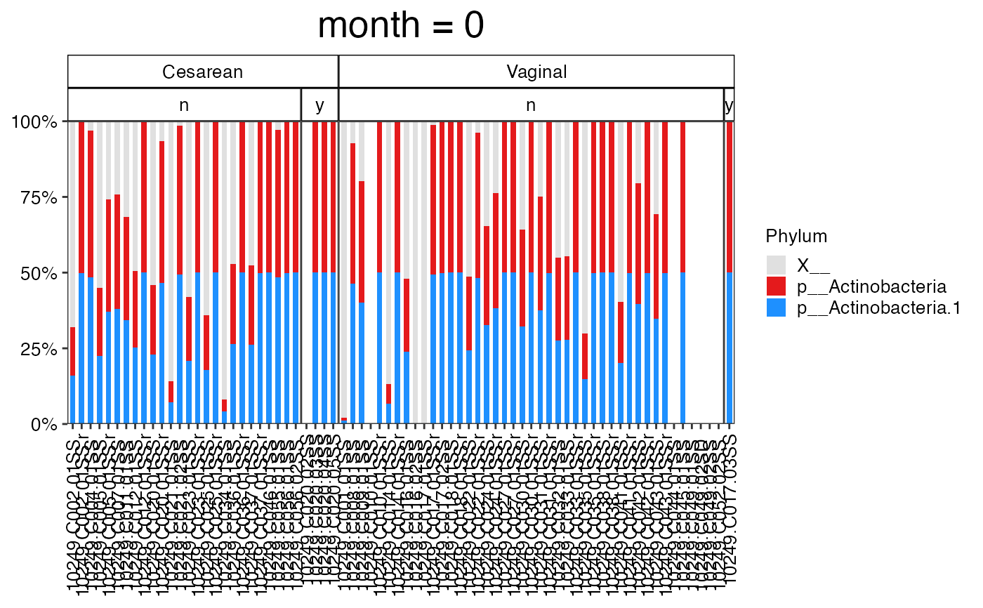
#> $Phylum
#> $Phylum$Phylum
#> $Phylum$Phylum$indiv
#> Warning: No shared levels found between `names(values)` of the manual scale and the
#> data's colour values.
 #>
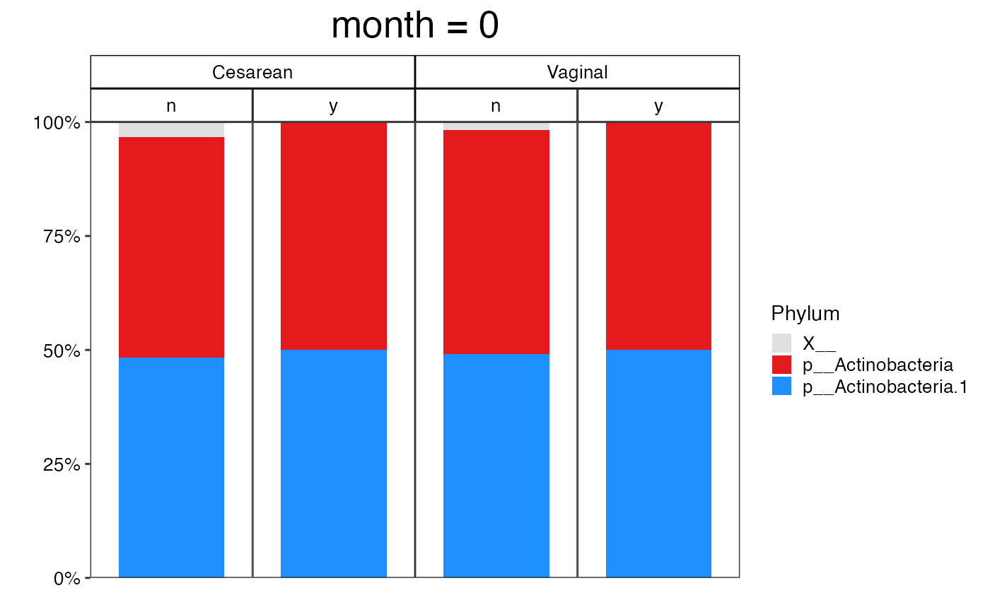
#> $Phylum$Phylum$average
#> Warning: No shared levels found between `names(values)` of the manual scale and the
#> data's colour values.
#>
#> $Phylum$Phylum$average
#> Warning: No shared levels found between `names(values)` of the manual scale and the
#> data's colour values.
 #>
#>
#>
plot_feature_diversity(
data.obj = ecam.obj,
group.var = "antiexposedall",
strata.var = "delivery",
time.var = "month",
time.point.plot = unique(ecam.obj$meta.dat$month)[1],
is.plot.change = TRUE,
feature.level = c("Phylum", "Family", "Genus"),
feature.dat.type = "proportion",
features.plot = NULL,
prop.to.lump = 0.0001,
top.k.plot = NULL,
top.k.func = NULL,
renormalize = FALSE,
plot.other = TRUE,
plot.scheme = "combined",
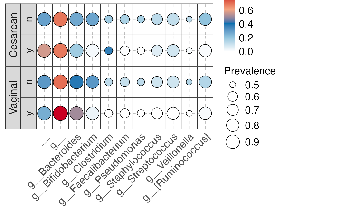
plot.type = "dotplot"
)
#> Validation passed.
#> Validation passed.
#> Data has been subsetted based on the provided samIDs.
#> Updated metadata to match the subsetted data.
#> 801 samples were excluded.
#> Updated feature table to match the subsetted data.
#> Feature annotation remains aligned to the current feature set.
#> Data subsetting complete. Returning updated data object.
#> Validation passed.
#> Validation passed.
#> Data has been subsetted based on the provided samIDs.
#> Updated metadata to match the subsetted data.
#> 801 samples were excluded.
#> Updated feature table to match the subsetted data.
#> Feature annotation remains aligned to the current feature set.
#> Data subsetting complete. Returning updated data object.
#> Validation passed.
#> Validation passed.
#> Data has been subsetted based on the provided samIDs.
#> Updated metadata to match the subsetted data.
#> 801 samples were excluded.
#> Updated feature table to match the subsetted data.
#> Feature annotation remains aligned to the current feature set.
#> Data subsetting complete. Returning updated data object.
#> $Phylum
#> $Phylum$Phylum
#>
#>
#>
plot_feature_diversity(
data.obj = ecam.obj,
group.var = "antiexposedall",
strata.var = "delivery",
time.var = "month",
time.point.plot = unique(ecam.obj$meta.dat$month)[1],
is.plot.change = TRUE,
feature.level = c("Phylum", "Family", "Genus"),
feature.dat.type = "proportion",
features.plot = NULL,
prop.to.lump = 0.0001,
top.k.plot = NULL,
top.k.func = NULL,
renormalize = FALSE,
plot.other = TRUE,
plot.scheme = "combined",
plot.type = "dotplot"
)
#> Validation passed.
#> Validation passed.
#> Data has been subsetted based on the provided samIDs.
#> Updated metadata to match the subsetted data.
#> 801 samples were excluded.
#> Updated feature table to match the subsetted data.
#> Feature annotation remains aligned to the current feature set.
#> Data subsetting complete. Returning updated data object.
#> Validation passed.
#> Validation passed.
#> Data has been subsetted based on the provided samIDs.
#> Updated metadata to match the subsetted data.
#> 801 samples were excluded.
#> Updated feature table to match the subsetted data.
#> Feature annotation remains aligned to the current feature set.
#> Data subsetting complete. Returning updated data object.
#> Validation passed.
#> Validation passed.
#> Data has been subsetted based on the provided samIDs.
#> Updated metadata to match the subsetted data.
#> 801 samples were excluded.
#> Updated feature table to match the subsetted data.
#> Feature annotation remains aligned to the current feature set.
#> Data subsetting complete. Returning updated data object.
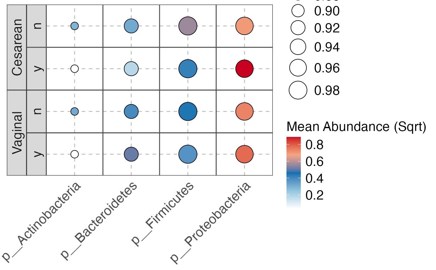
#> $Phylum
#> $Phylum$Phylum
 #>
#>
#> $Family
#> $Family$Family
#>
#>
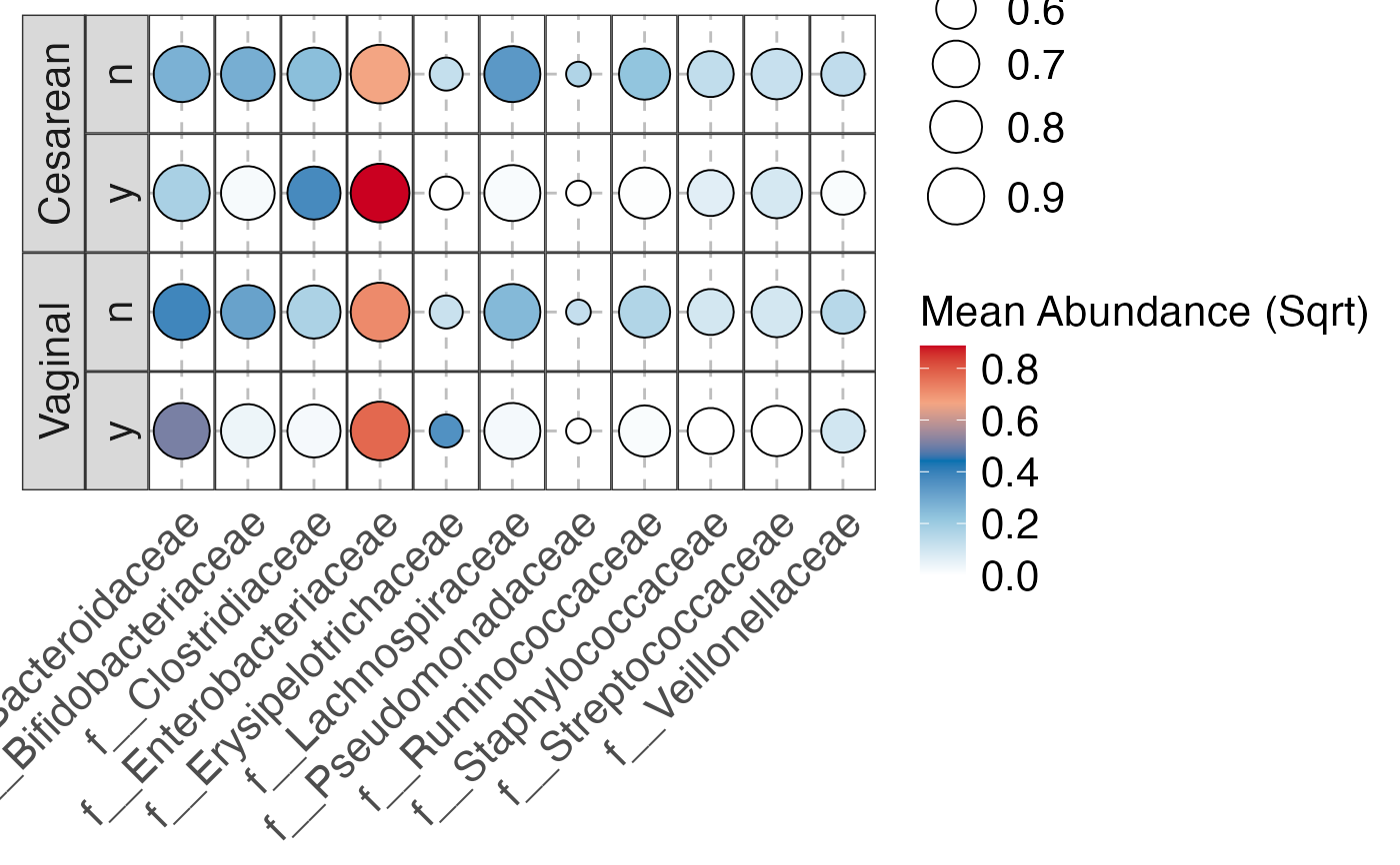
#> $Family
#> $Family$Family
 #>
#>
#> $Genus
#> $Genus$Genus
#>
#>
#> $Genus
#> $Genus$Genus
 #>
#>
plot_feature_diversity(
data.obj = ecam.obj,
group.var = "antiexposedall",
strata.var = "delivery",
time.var = "month",
time.point.plot = unique(ecam.obj$meta.dat$month)[1],
is.plot.change = TRUE,
feature.level = c("Phylum", "Family", "Genus"),
feature.dat.type = "proportion",
features.plot = NULL,
prop.to.lump = 0.0001,
top.k.plot = NULL,
top.k.func = NULL,
renormalize = FALSE,
plot.other = TRUE,
plot.scheme = "combined",
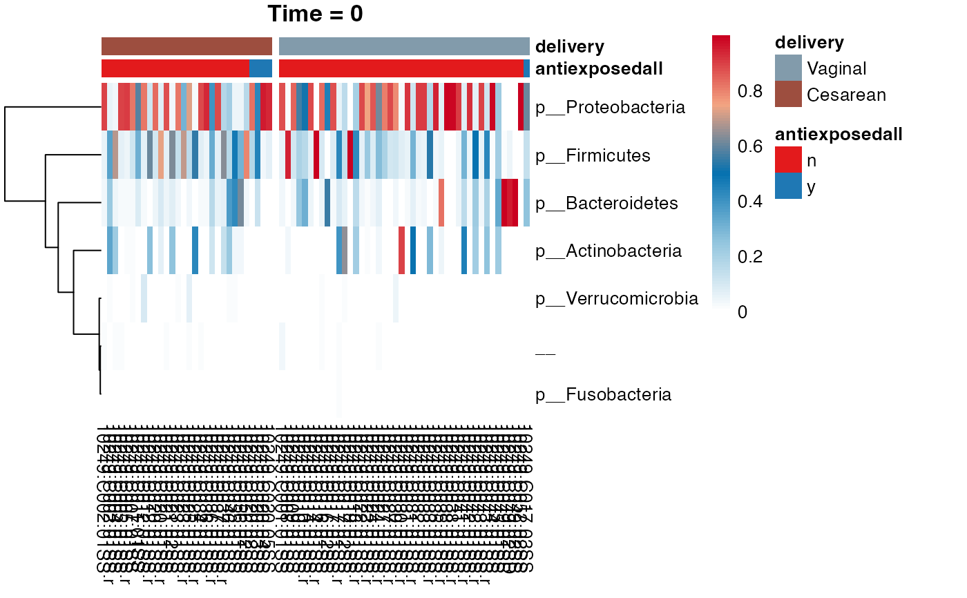
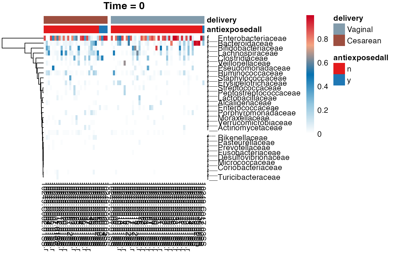
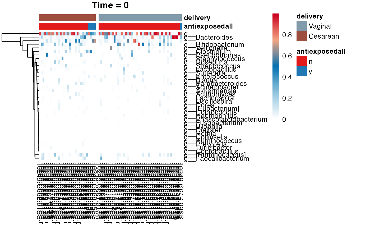
plot.type = "heatmap"
)
#> Validation passed.
#> Validation passed.
#> Data has been subsetted based on the provided samIDs.
#> Updated metadata to match the subsetted data.
#> 801 samples were excluded.
#> Updated feature table to match the subsetted data.
#> Feature annotation remains aligned to the current feature set.
#> Data subsetting complete. Returning updated data object.
#> Validation passed.
#> Validation passed.
#> Data has been subsetted based on the provided samIDs.
#> Updated metadata to match the subsetted data.
#> 801 samples were excluded.
#> Updated feature table to match the subsetted data.
#> Feature annotation remains aligned to the current feature set.
#> Data subsetting complete. Returning updated data object.
#> Validation passed.
#> Validation passed.
#> Data has been subsetted based on the provided samIDs.
#> Updated metadata to match the subsetted data.
#> 801 samples were excluded.
#> Updated feature table to match the subsetted data.
#> Feature annotation remains aligned to the current feature set.
#> Data subsetting complete. Returning updated data object.
#> $Phylum
#> $Phylum$Phylum
#>
#>
plot_feature_diversity(
data.obj = ecam.obj,
group.var = "antiexposedall",
strata.var = "delivery",
time.var = "month",
time.point.plot = unique(ecam.obj$meta.dat$month)[1],
is.plot.change = TRUE,
feature.level = c("Phylum", "Family", "Genus"),
feature.dat.type = "proportion",
features.plot = NULL,
prop.to.lump = 0.0001,
top.k.plot = NULL,
top.k.func = NULL,
renormalize = FALSE,
plot.other = TRUE,
plot.scheme = "combined",
plot.type = "heatmap"
)
#> Validation passed.
#> Validation passed.
#> Data has been subsetted based on the provided samIDs.
#> Updated metadata to match the subsetted data.
#> 801 samples were excluded.
#> Updated feature table to match the subsetted data.
#> Feature annotation remains aligned to the current feature set.
#> Data subsetting complete. Returning updated data object.
#> Validation passed.
#> Validation passed.
#> Data has been subsetted based on the provided samIDs.
#> Updated metadata to match the subsetted data.
#> 801 samples were excluded.
#> Updated feature table to match the subsetted data.
#> Feature annotation remains aligned to the current feature set.
#> Data subsetting complete. Returning updated data object.
#> Validation passed.
#> Validation passed.
#> Data has been subsetted based on the provided samIDs.
#> Updated metadata to match the subsetted data.
#> 801 samples were excluded.
#> Updated feature table to match the subsetted data.
#> Feature annotation remains aligned to the current feature set.
#> Data subsetting complete. Returning updated data object.
#> $Phylum
#> $Phylum$Phylum
 #>
#>
#> $Family
#> $Family$Family
#>
#>
#> $Family
#> $Family$Family
 #>
#>
#> $Genus
#> $Genus$Genus
#>
#>
#> $Genus
#> $Genus$Genus
 #>
#>
plot_feature_diversity(
data.obj = ecam.obj,
group.var = "antiexposedall",
strata.var = "delivery",
time.var = "month",
time.point.plot = unique(ecam.obj$meta.dat$month)[1],
is.plot.change = TRUE,
feature.level = c("Phylum", "Family", "Genus"),
feature.dat.type = "proportion",
features.plot = NULL,
prop.to.lump = 0.0001,
top.k.plot = NULL,
top.k.func = NULL,
renormalize = FALSE,
plot.other = TRUE,
plot.scheme = "combined",
plot.type = "boxplot"
)
#> Validation passed.
#> Validation passed.
#> Data has been subsetted based on the provided samIDs.
#> Updated metadata to match the subsetted data.
#> 801 samples were excluded.
#> Updated feature table to match the subsetted data.
#> Feature annotation remains aligned to the current feature set.
#> Data subsetting complete. Returning updated data object.
#> Validation passed.
#> Validation passed.
#> Data has been subsetted based on the provided samIDs.
#> Updated metadata to match the subsetted data.
#> 801 samples were excluded.
#> Updated feature table to match the subsetted data.
#> Feature annotation remains aligned to the current feature set.
#> Data subsetting complete. Returning updated data object.
#> Validation passed.
#> Validation passed.
#> Data has been subsetted based on the provided samIDs.
#> Updated metadata to match the subsetted data.
#> 801 samples were excluded.
#> Updated feature table to match the subsetted data.
#> Feature annotation remains aligned to the current feature set.
#> Data subsetting complete. Returning updated data object.
#> $Phylum
#> $Phylum$Phylum
#>
#>
plot_feature_diversity(
data.obj = ecam.obj,
group.var = "antiexposedall",
strata.var = "delivery",
time.var = "month",
time.point.plot = unique(ecam.obj$meta.dat$month)[1],
is.plot.change = TRUE,
feature.level = c("Phylum", "Family", "Genus"),
feature.dat.type = "proportion",
features.plot = NULL,
prop.to.lump = 0.0001,
top.k.plot = NULL,
top.k.func = NULL,
renormalize = FALSE,
plot.other = TRUE,
plot.scheme = "combined",
plot.type = "boxplot"
)
#> Validation passed.
#> Validation passed.
#> Data has been subsetted based on the provided samIDs.
#> Updated metadata to match the subsetted data.
#> 801 samples were excluded.
#> Updated feature table to match the subsetted data.
#> Feature annotation remains aligned to the current feature set.
#> Data subsetting complete. Returning updated data object.
#> Validation passed.
#> Validation passed.
#> Data has been subsetted based on the provided samIDs.
#> Updated metadata to match the subsetted data.
#> 801 samples were excluded.
#> Updated feature table to match the subsetted data.
#> Feature annotation remains aligned to the current feature set.
#> Data subsetting complete. Returning updated data object.
#> Validation passed.
#> Validation passed.
#> Data has been subsetted based on the provided samIDs.
#> Updated metadata to match the subsetted data.
#> 801 samples were excluded.
#> Updated feature table to match the subsetted data.
#> Feature annotation remains aligned to the current feature set.
#> Data subsetting complete. Returning updated data object.
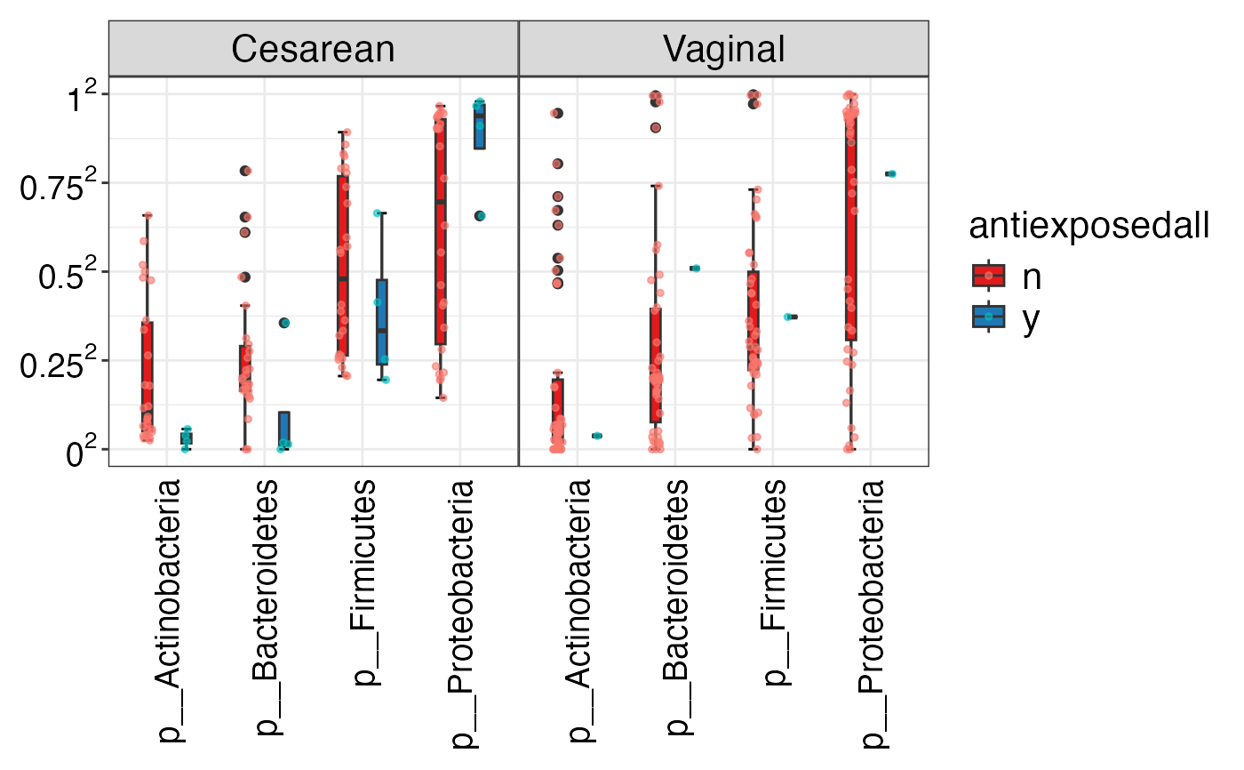
#> $Phylum
#> $Phylum$Phylum
 #>
#>
#> $Family
#> $Family$Family
#>
#>
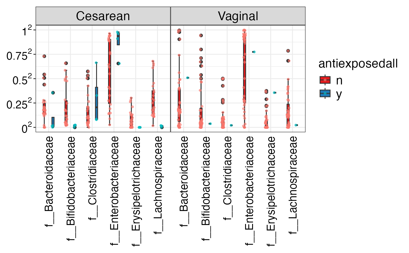
#> $Family
#> $Family$Family
 #>
#>
#> $Genus
#> $Genus$Genus
#>
#>
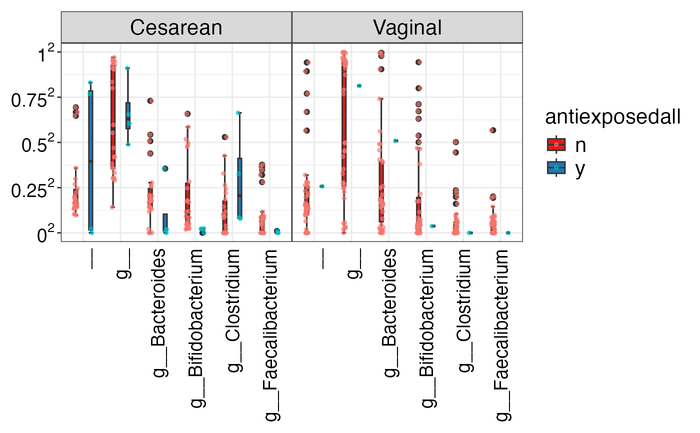
#> $Genus
#> $Genus$Genus
 #>
#>
plot_feature_diversity(
data.obj = ecam.obj,
group.var = "antiexposedall",
strata.var = "delivery",
time.var = "month",
time.point.plot = unique(ecam.obj$meta.dat$month)[1],
is.plot.change = TRUE,
feature.level = c("Phylum", "Family", "Genus"),
feature.dat.type = "proportion",
features.plot = NULL,
prop.to.lump = 0.0001,
top.k.plot = NULL,
top.k.func = NULL,
renormalize = FALSE,
plot.other = TRUE,
plot.scheme = "individual",
plot.type = "boxplot"
)
#> Validation passed.
#> Validation passed.
#> Data has been subsetted based on the provided samIDs.
#> Updated metadata to match the subsetted data.
#> 801 samples were excluded.
#> Updated feature table to match the subsetted data.
#> Feature annotation remains aligned to the current feature set.
#> Data subsetting complete. Returning updated data object.
#> Validation passed.
#> Validation passed.
#> Data has been subsetted based on the provided samIDs.
#> Updated metadata to match the subsetted data.
#> 801 samples were excluded.
#> Updated feature table to match the subsetted data.
#> Feature annotation remains aligned to the current feature set.
#> Data subsetting complete. Returning updated data object.
#> Validation passed.
#> Validation passed.
#> Data has been subsetted based on the provided samIDs.
#> Updated metadata to match the subsetted data.
#> 801 samples were excluded.
#> Updated feature table to match the subsetted data.
#> Feature annotation remains aligned to the current feature set.
#> Data subsetting complete. Returning updated data object.
#> $Phylum
#> $Phylum$Phylum
#> $Phylum$Phylum$p__Actinobacteria
#>
#>
plot_feature_diversity(
data.obj = ecam.obj,
group.var = "antiexposedall",
strata.var = "delivery",
time.var = "month",
time.point.plot = unique(ecam.obj$meta.dat$month)[1],
is.plot.change = TRUE,
feature.level = c("Phylum", "Family", "Genus"),
feature.dat.type = "proportion",
features.plot = NULL,
prop.to.lump = 0.0001,
top.k.plot = NULL,
top.k.func = NULL,
renormalize = FALSE,
plot.other = TRUE,
plot.scheme = "individual",
plot.type = "boxplot"
)
#> Validation passed.
#> Validation passed.
#> Data has been subsetted based on the provided samIDs.
#> Updated metadata to match the subsetted data.
#> 801 samples were excluded.
#> Updated feature table to match the subsetted data.
#> Feature annotation remains aligned to the current feature set.
#> Data subsetting complete. Returning updated data object.
#> Validation passed.
#> Validation passed.
#> Data has been subsetted based on the provided samIDs.
#> Updated metadata to match the subsetted data.
#> 801 samples were excluded.
#> Updated feature table to match the subsetted data.
#> Feature annotation remains aligned to the current feature set.
#> Data subsetting complete. Returning updated data object.
#> Validation passed.
#> Validation passed.
#> Data has been subsetted based on the provided samIDs.
#> Updated metadata to match the subsetted data.
#> 801 samples were excluded.
#> Updated feature table to match the subsetted data.
#> Feature annotation remains aligned to the current feature set.
#> Data subsetting complete. Returning updated data object.
#> $Phylum
#> $Phylum$Phylum
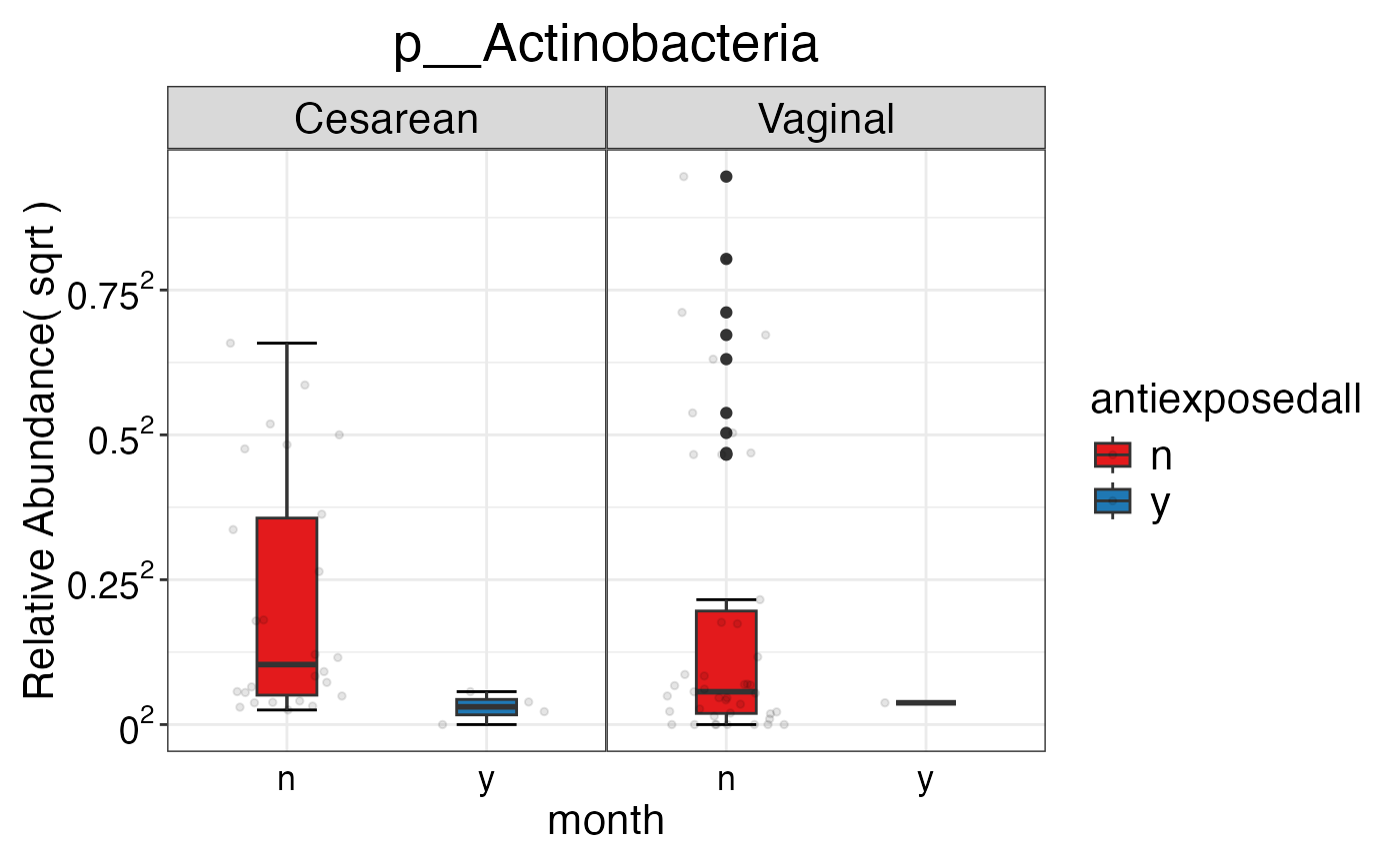
#> $Phylum$Phylum$p__Actinobacteria
 #>
#> $Phylum$Phylum$p__Bacteroidetes
#>
#> $Phylum$Phylum$p__Bacteroidetes
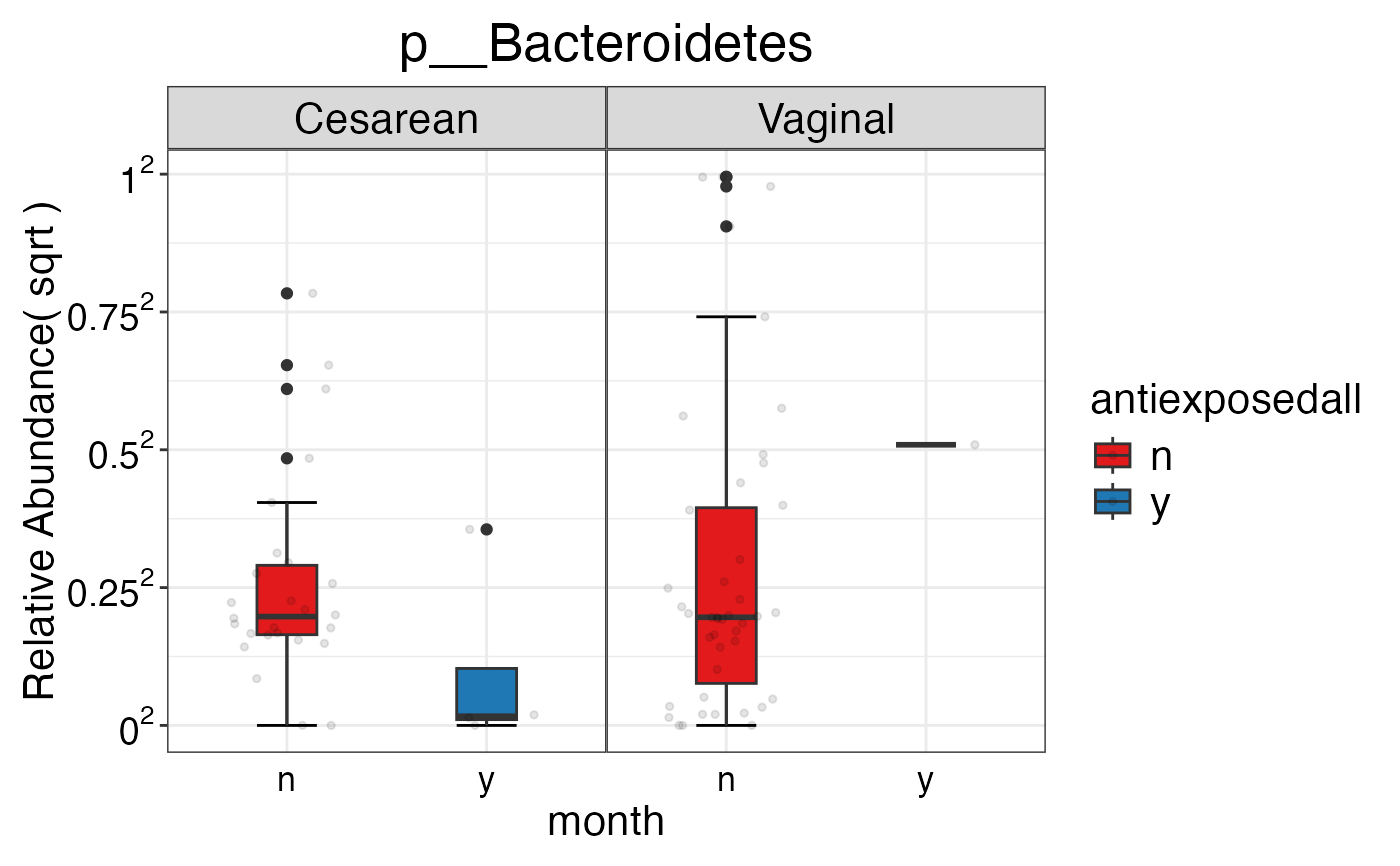 #>
#> $Phylum$Phylum$p__Firmicutes
#>
#> $Phylum$Phylum$p__Firmicutes
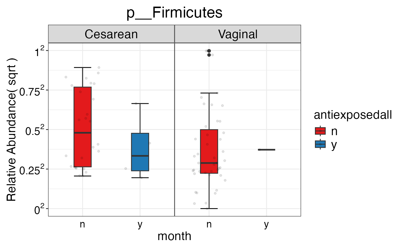 #>
#> $Phylum$Phylum$p__Proteobacteria
#>
#> $Phylum$Phylum$p__Proteobacteria
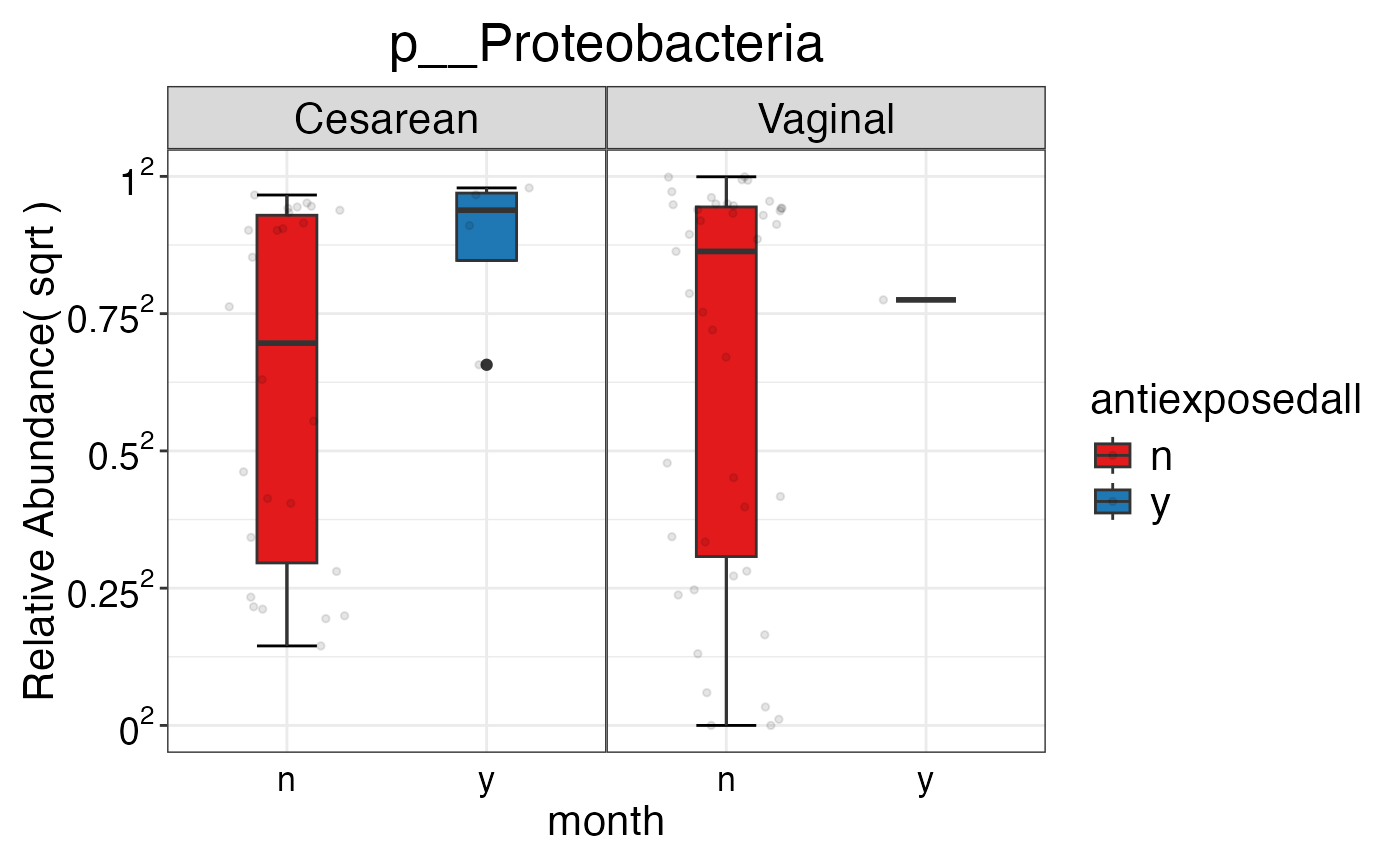 #>
#>
#>
#> $Family
#> $Family$Family
#> $Family$Family$f__Bacteroidaceae
#>
#>
#>
#> $Family
#> $Family$Family
#> $Family$Family$f__Bacteroidaceae
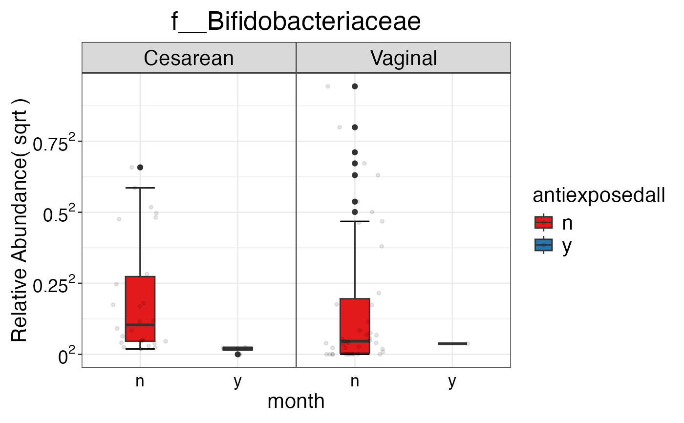
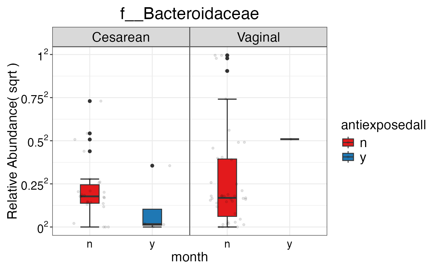 #>
#> $Family$Family$f__Bifidobacteriaceae
#>
#> $Family$Family$f__Bifidobacteriaceae
 #>
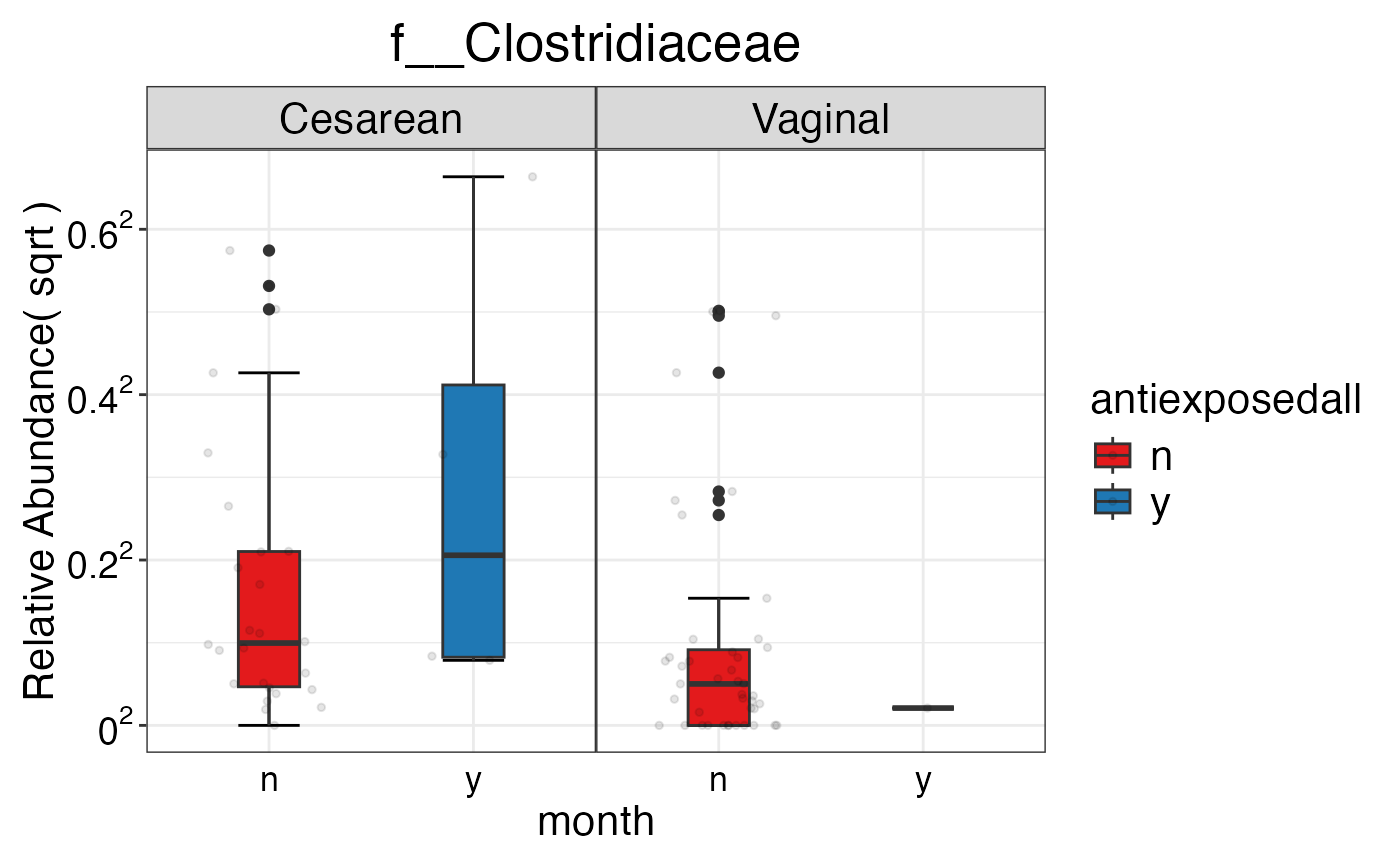
#> $Family$Family$f__Clostridiaceae
#>
#> $Family$Family$f__Clostridiaceae
 #>
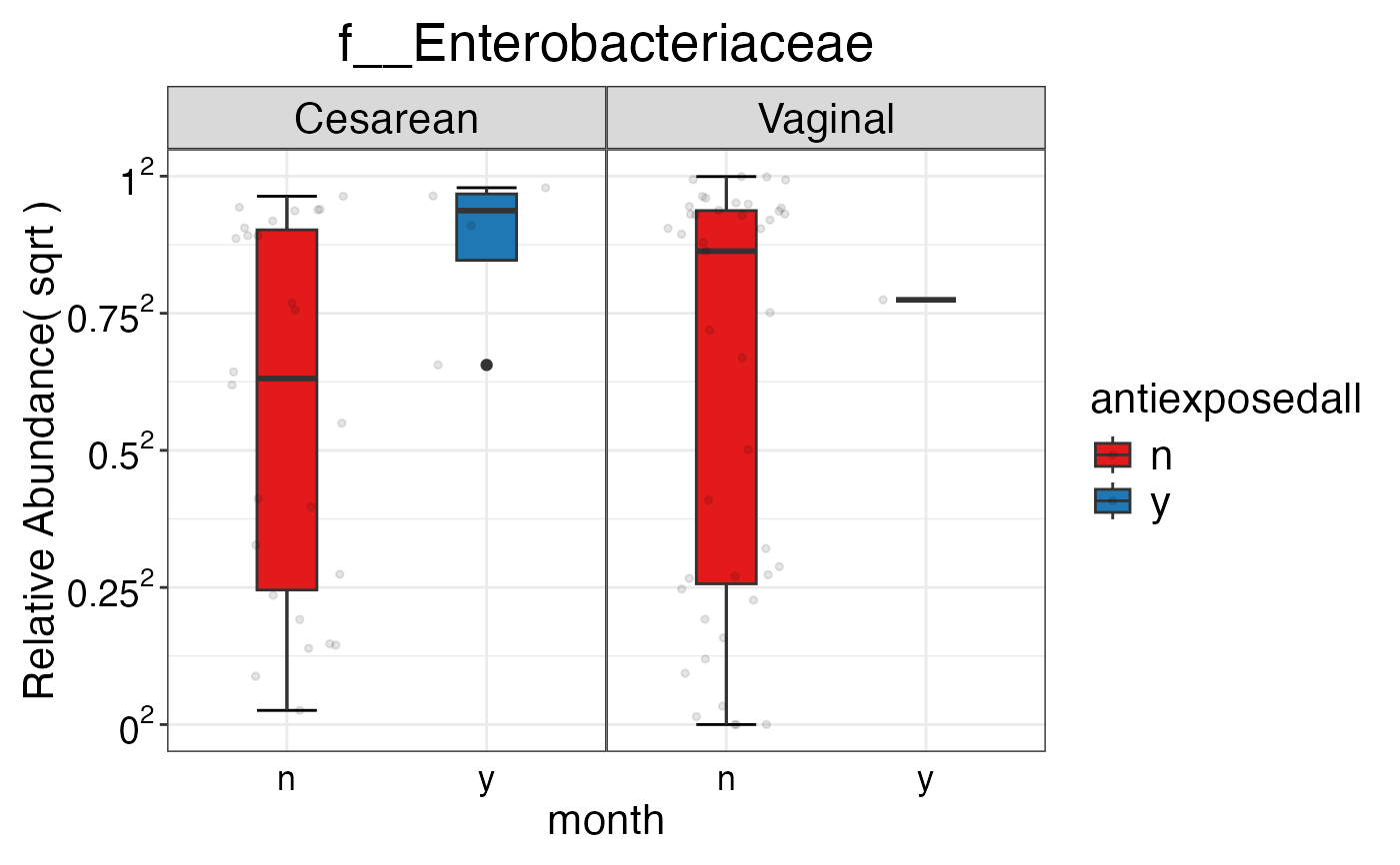
#> $Family$Family$f__Enterobacteriaceae
#>
#> $Family$Family$f__Enterobacteriaceae
 #>
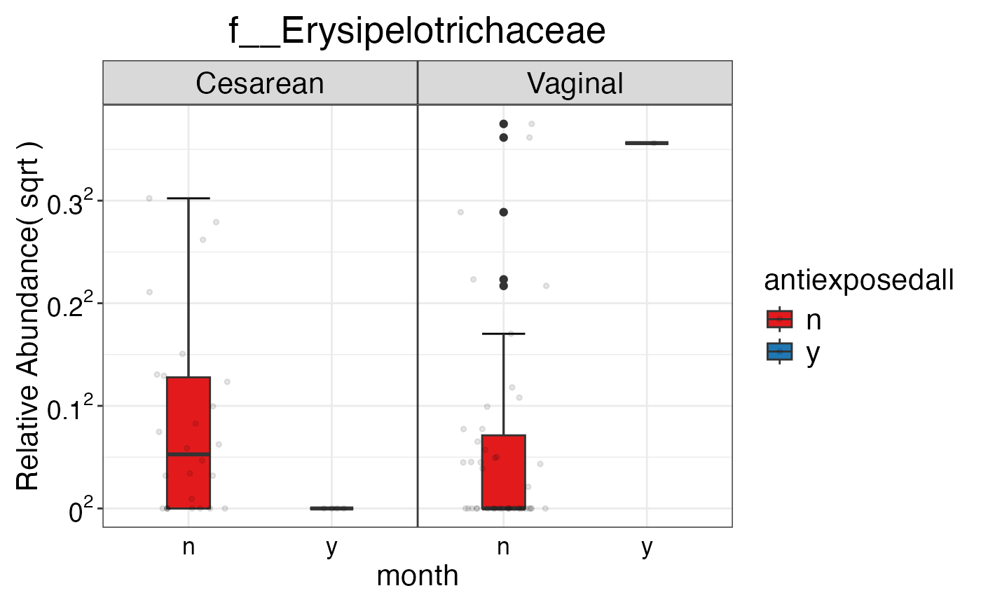
#> $Family$Family$f__Erysipelotrichaceae
#>
#> $Family$Family$f__Erysipelotrichaceae
 #>
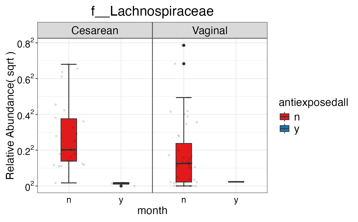
#> $Family$Family$f__Lachnospiraceae
#>
#> $Family$Family$f__Lachnospiraceae
 #>
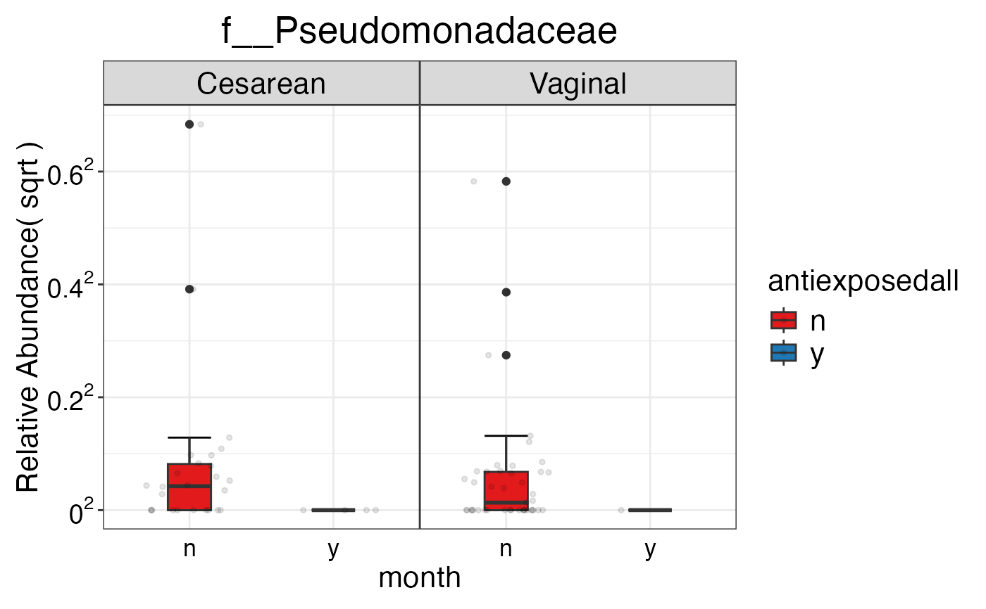
#> $Family$Family$f__Pseudomonadaceae
#>
#> $Family$Family$f__Pseudomonadaceae
 #>
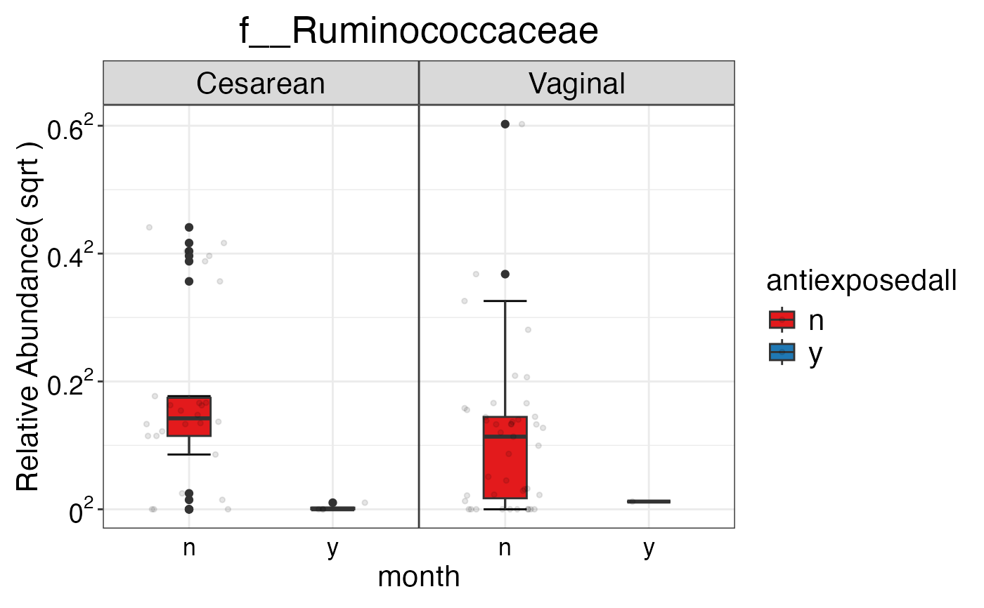
#> $Family$Family$f__Ruminococcaceae
#>
#> $Family$Family$f__Ruminococcaceae
 #>
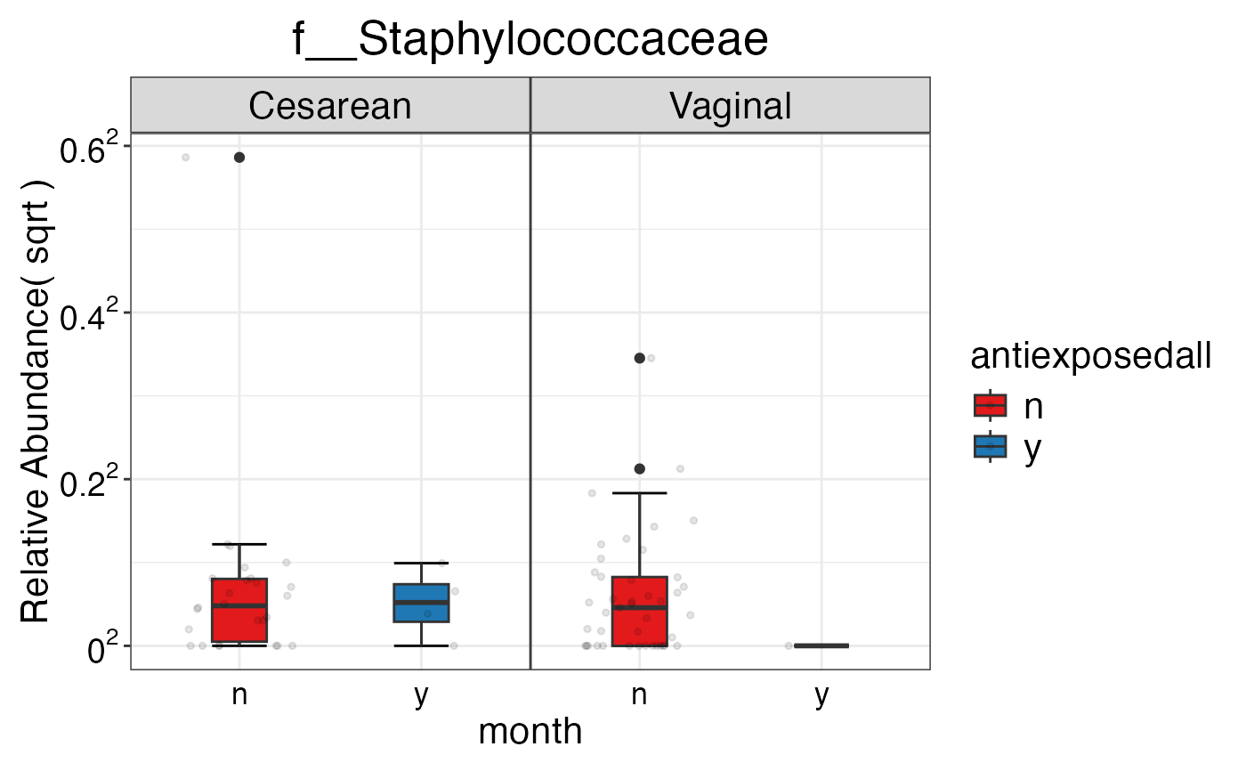
#> $Family$Family$f__Staphylococcaceae
#>
#> $Family$Family$f__Staphylococcaceae
 #>
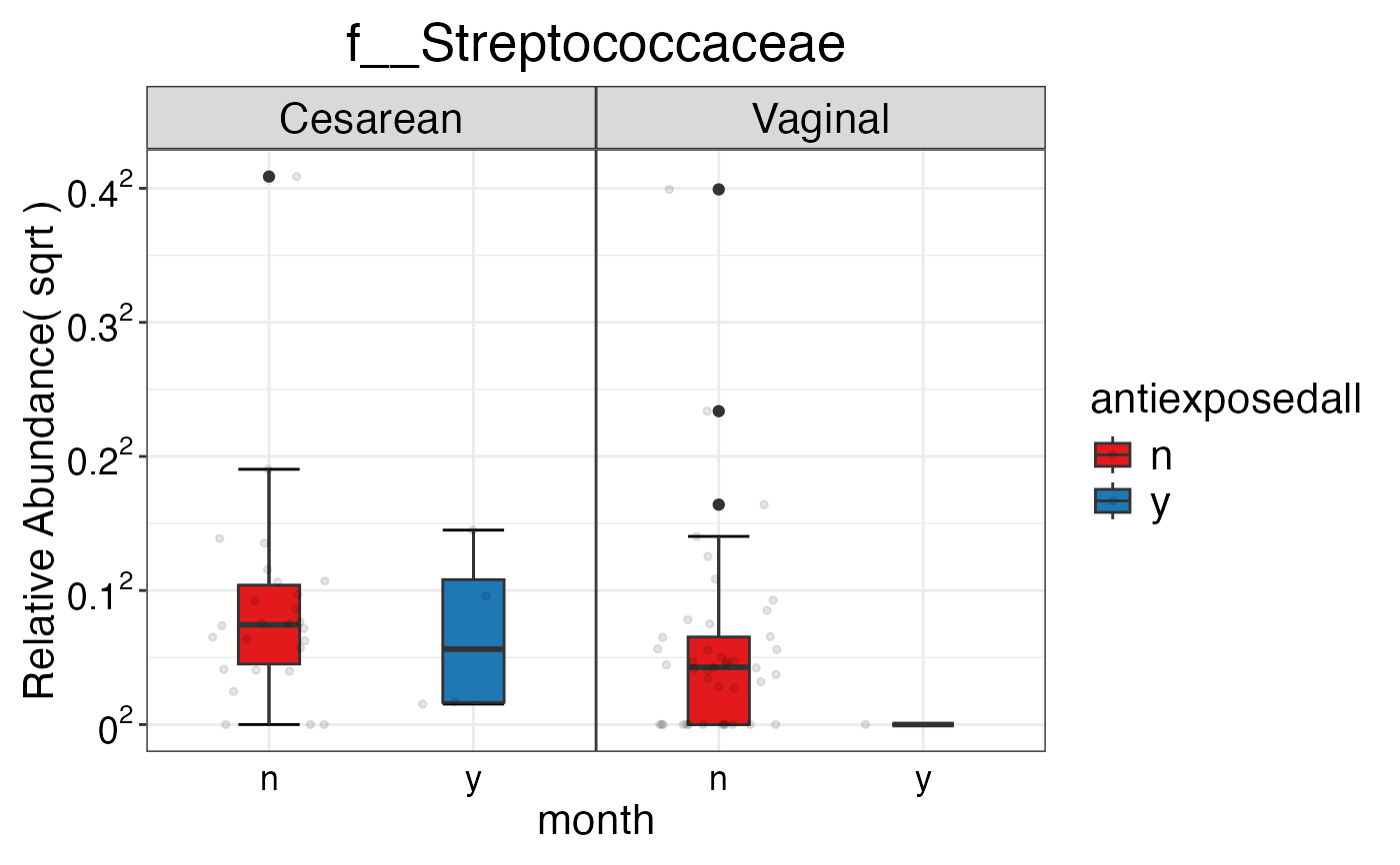
#> $Family$Family$f__Streptococcaceae
#>
#> $Family$Family$f__Streptococcaceae
 #>
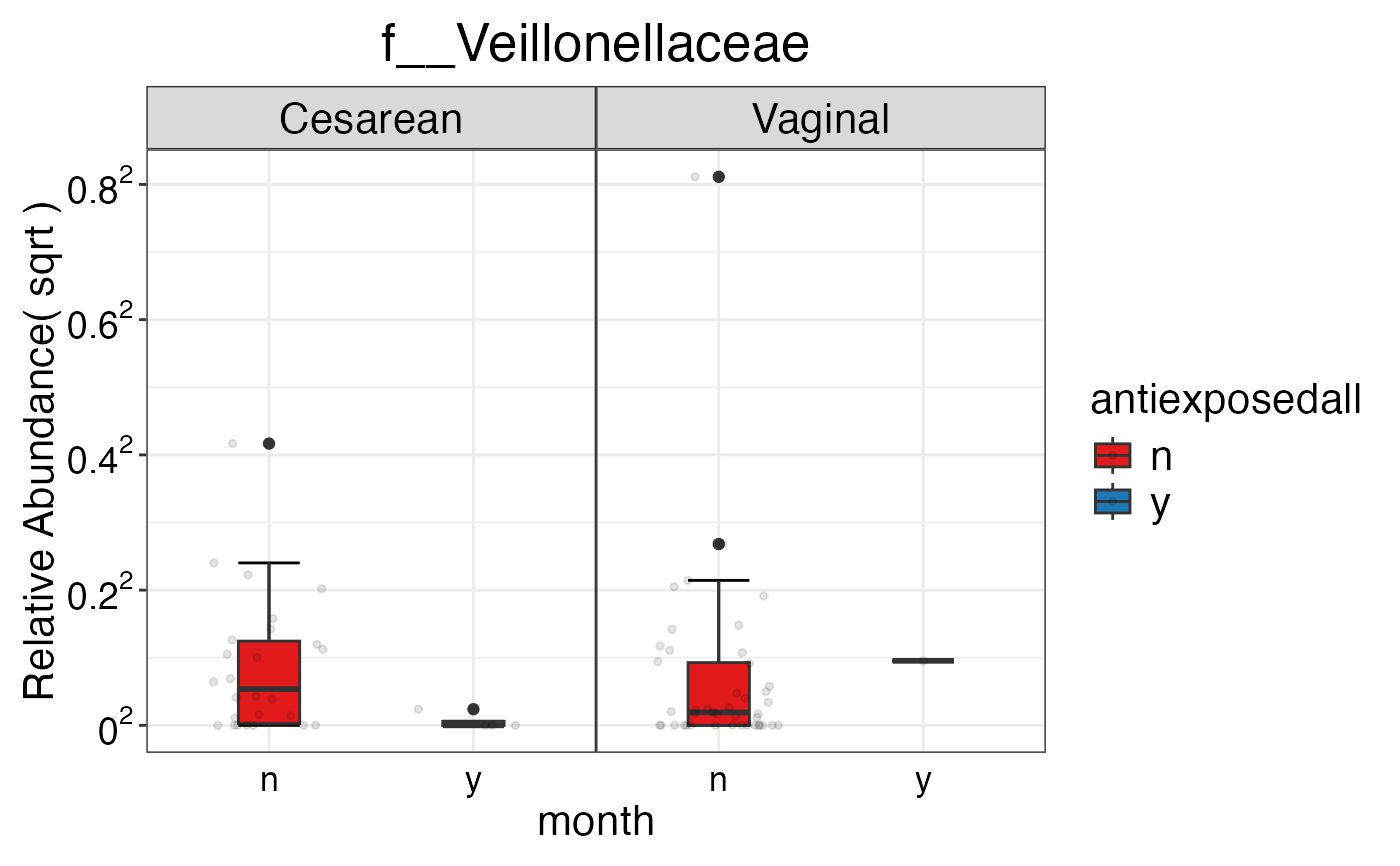
#> $Family$Family$f__Veillonellaceae
#>
#> $Family$Family$f__Veillonellaceae
 #>
#>
#>
#> $Genus
#> $Genus$Genus
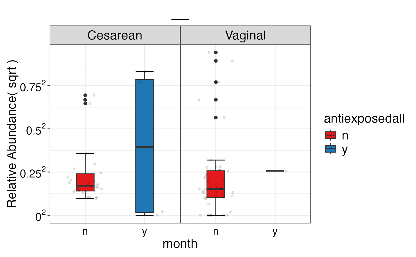
#> $Genus$Genus$`__`
#>
#>
#>
#> $Genus
#> $Genus$Genus
#> $Genus$Genus$`__`
 #>
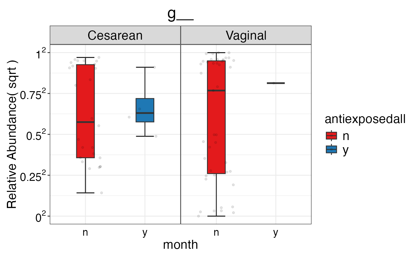
#> $Genus$Genus$g__
#>
#> $Genus$Genus$g__
 #>
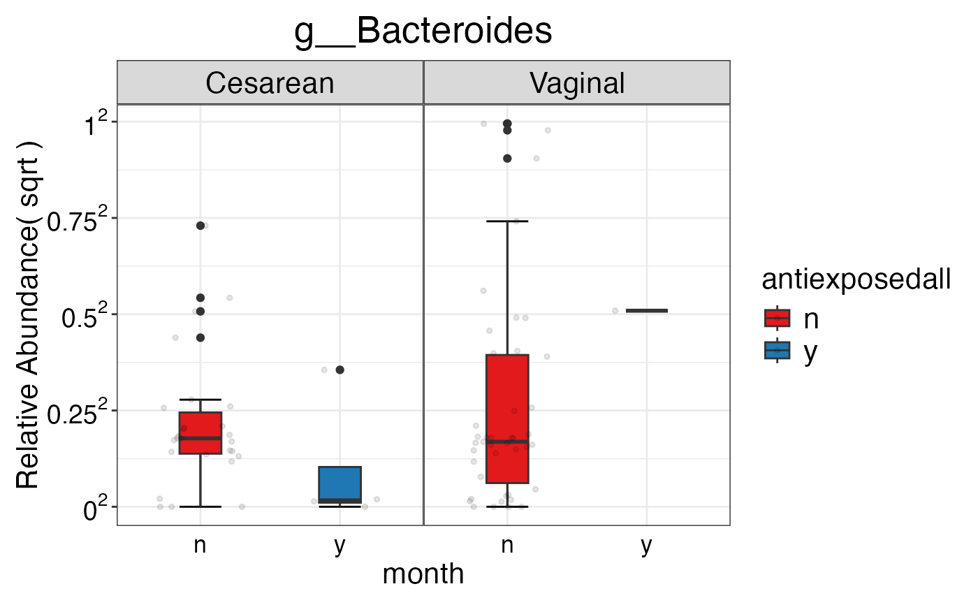
#> $Genus$Genus$g__Bacteroides
#>
#> $Genus$Genus$g__Bacteroides
 #>
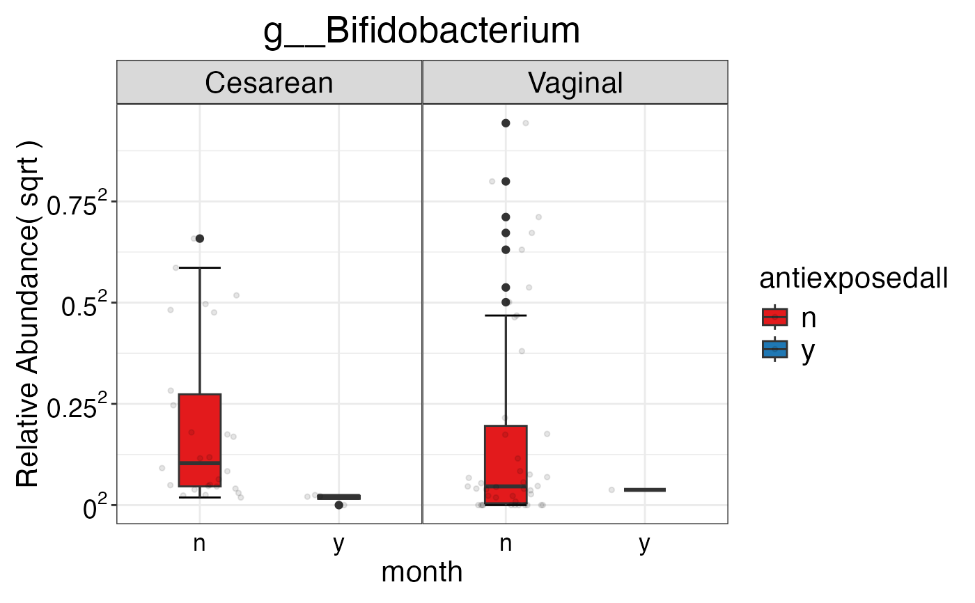
#> $Genus$Genus$g__Bifidobacterium
#>
#> $Genus$Genus$g__Bifidobacterium
 #>
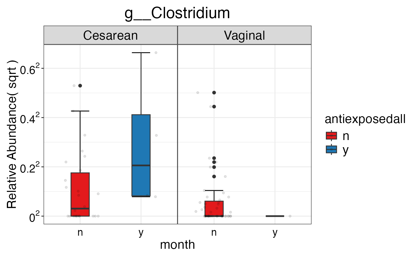
#> $Genus$Genus$g__Clostridium
#>
#> $Genus$Genus$g__Clostridium
 #>
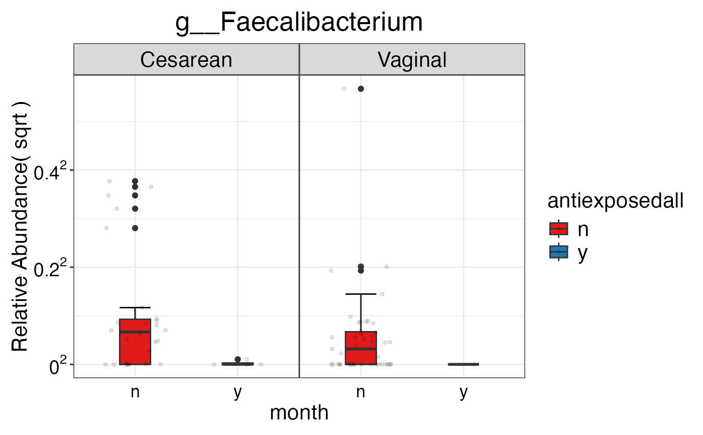
#> $Genus$Genus$g__Faecalibacterium
#>
#> $Genus$Genus$g__Faecalibacterium
 #>
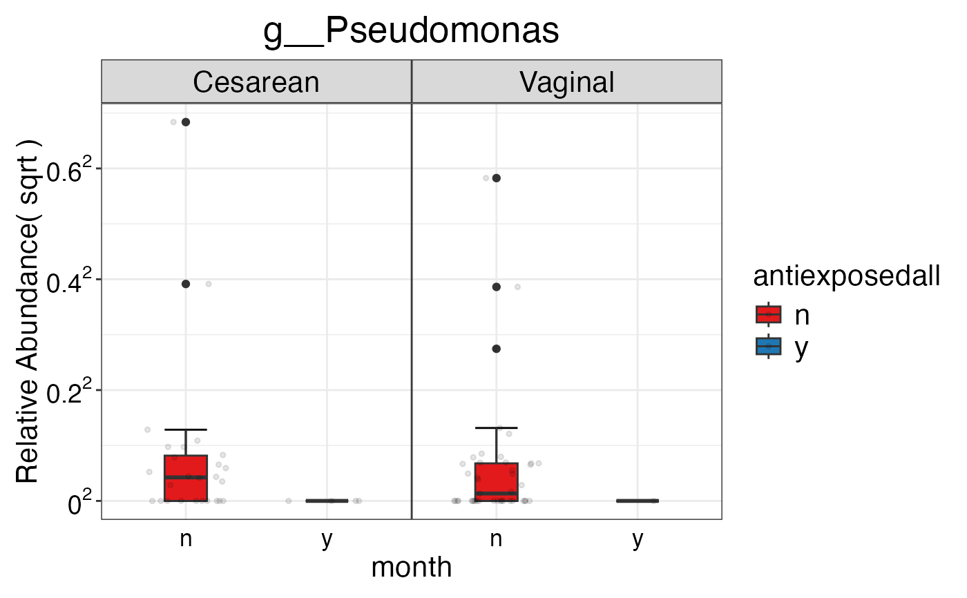
#> $Genus$Genus$g__Pseudomonas
#>
#> $Genus$Genus$g__Pseudomonas
 #>
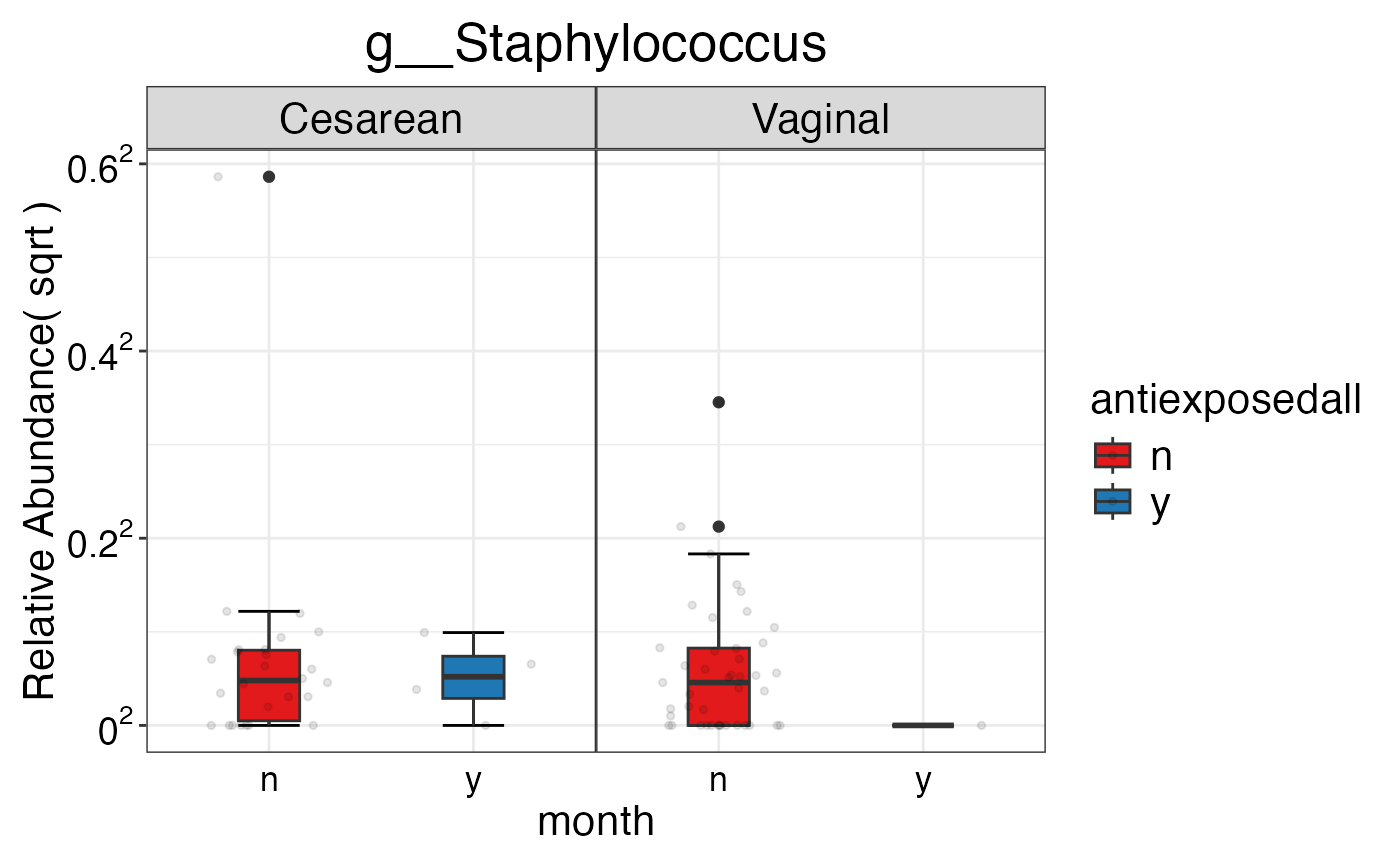
#> $Genus$Genus$g__Staphylococcus
#>
#> $Genus$Genus$g__Staphylococcus
 #>
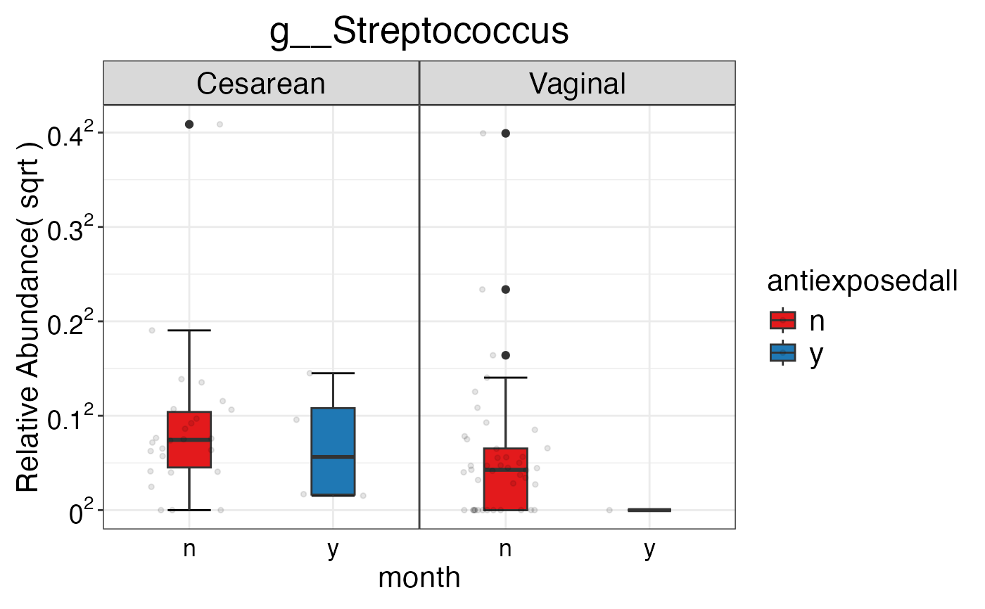
#> $Genus$Genus$g__Streptococcus
#>
#> $Genus$Genus$g__Streptococcus
 #>
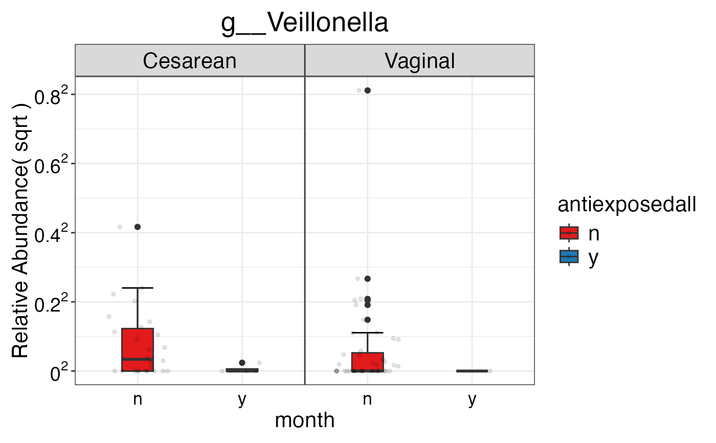
#> $Genus$Genus$g__Veillonella
#>
#> $Genus$Genus$g__Veillonella
 #>
#> $Genus$Genus$`g__[Ruminococcus]`
#>
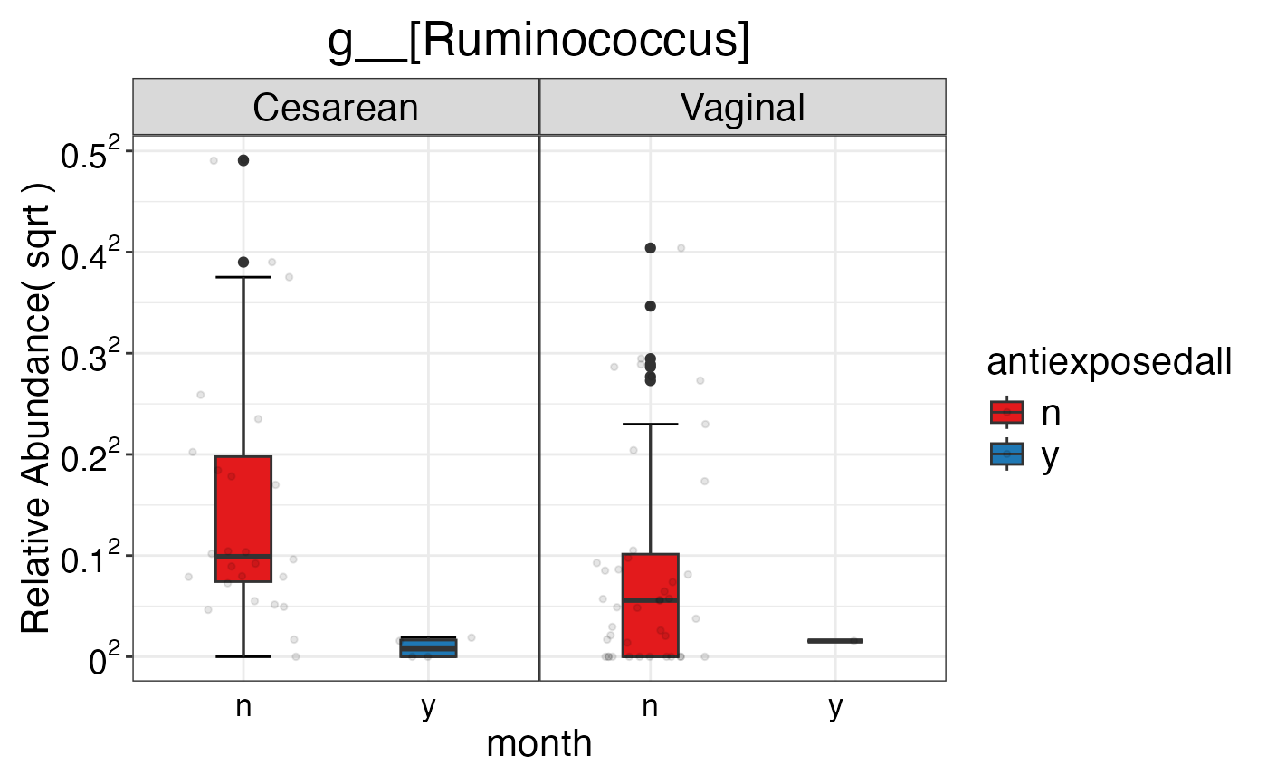
#> $Genus$Genus$`g__[Ruminococcus]`
 #>
#>
#>
data(peerj32.obj)
plot_feature_diversity(
data.obj = peerj32.obj,
group.var = "group",
strata.var = "sex",
subject.var = "subject",
time.var = "time",
time.point.plot = c("1", "2"),
is.plot.change = TRUE,
feature.change.func = "relative change",
feature.level = c("Phylum", "Family", "Genus"),
prop.to.lump = 0.0001,
top.k.plot = NULL,
top.k.func = NULL,
renormalize = FALSE,
plot.other = TRUE,
plot.scheme = "combined",
plot.type = "boxplot"
)
#> Validation passed.
#> Your data is in raw format ('Raw'). Normalization is crucial for further analyses. Now, 'mStat_normalize_data' function is automatically applying 'TSS' transformation.
#> Data has been successfully normalized using TSS method.
#> Validation passed.
#> Your data is in raw format ('Raw'). Normalization is crucial for further analyses. Now, 'mStat_normalize_data' function is automatically applying 'TSS' transformation.
#> Data has been successfully normalized using TSS method.
#> Validation passed.
#> Your data is in raw format ('Raw'). Normalization is crucial for further analyses. Now, 'mStat_normalize_data' function is automatically applying 'TSS' transformation.
#> Data has been successfully normalized using TSS method.
#> $Phylum
#> $Phylum$Phylum
#>
#>
#>
data(peerj32.obj)
plot_feature_diversity(
data.obj = peerj32.obj,
group.var = "group",
strata.var = "sex",
subject.var = "subject",
time.var = "time",
time.point.plot = c("1", "2"),
is.plot.change = TRUE,
feature.change.func = "relative change",
feature.level = c("Phylum", "Family", "Genus"),
prop.to.lump = 0.0001,
top.k.plot = NULL,
top.k.func = NULL,
renormalize = FALSE,
plot.other = TRUE,
plot.scheme = "combined",
plot.type = "boxplot"
)
#> Validation passed.
#> Your data is in raw format ('Raw'). Normalization is crucial for further analyses. Now, 'mStat_normalize_data' function is automatically applying 'TSS' transformation.
#> Data has been successfully normalized using TSS method.
#> Validation passed.
#> Your data is in raw format ('Raw'). Normalization is crucial for further analyses. Now, 'mStat_normalize_data' function is automatically applying 'TSS' transformation.
#> Data has been successfully normalized using TSS method.
#> Validation passed.
#> Your data is in raw format ('Raw'). Normalization is crucial for further analyses. Now, 'mStat_normalize_data' function is automatically applying 'TSS' transformation.
#> Data has been successfully normalized using TSS method.
#> $Phylum
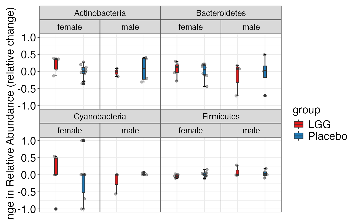
#> $Phylum$Phylum
 #>
#>
#> $Family
#> $Family$Family
#>
#>
#> $Family
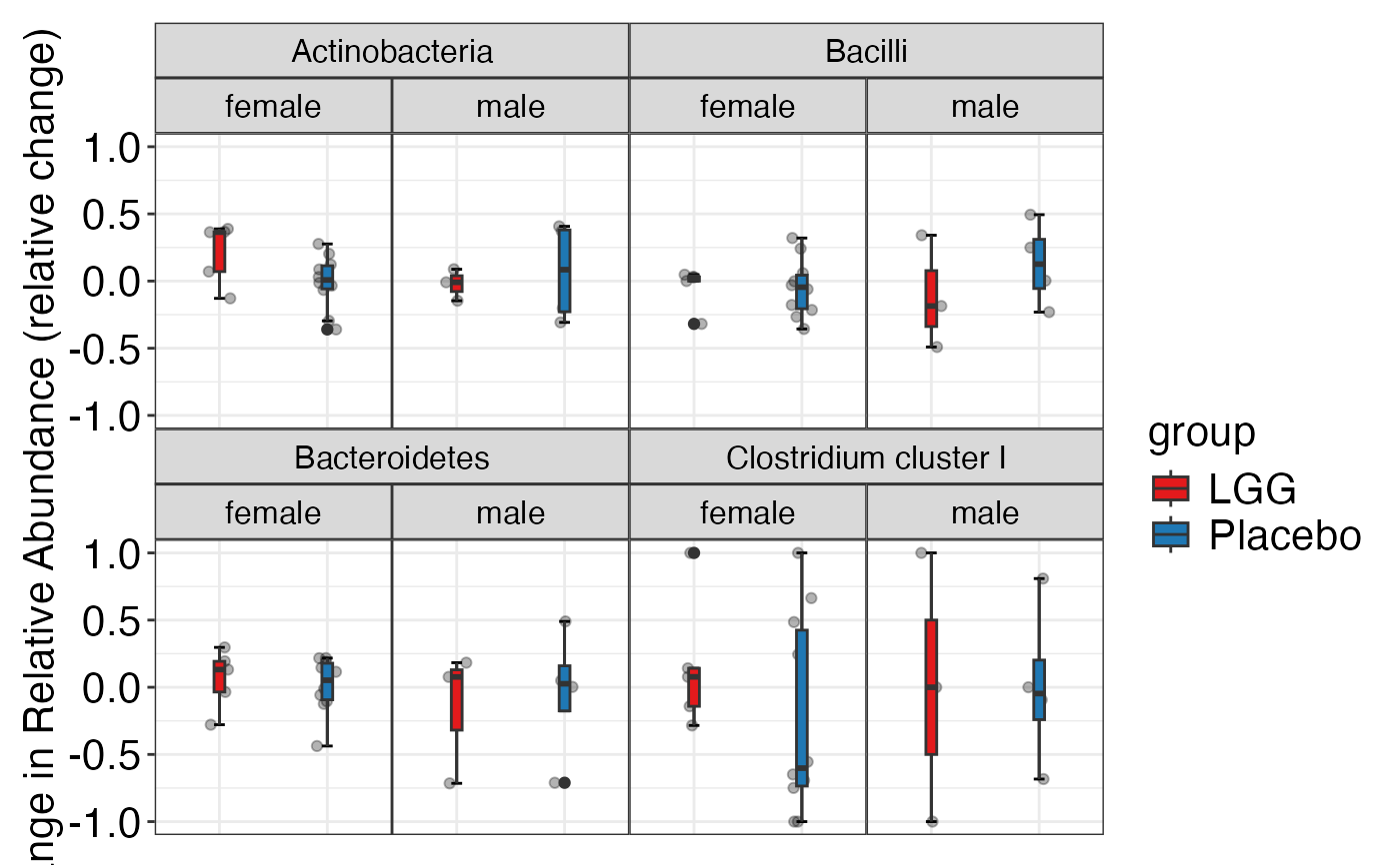
#> $Family$Family
 #>
#>
#> $Genus
#> $Genus$Genus
#>
#>
#> $Genus
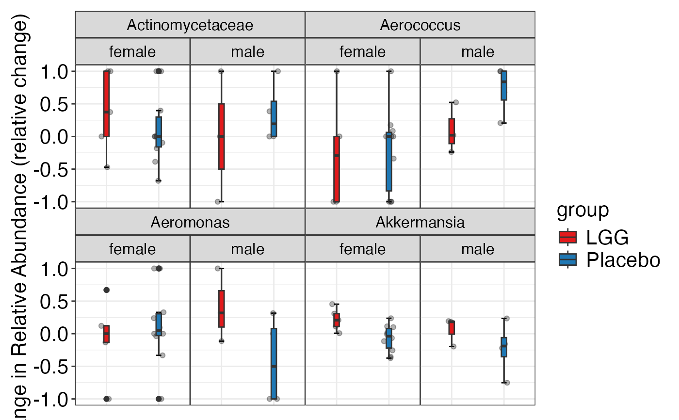
#> $Genus$Genus
 #>
#>
plot_feature_diversity(
data.obj = peerj32.obj,
group.var = "group",
strata.var = "sex",
subject.var = "subject",
time.var = "time",
time.point.plot = c("1", "2"),
is.plot.change = TRUE,
feature.change.func = "relative change",
feature.level = c("Phylum", "Family", "Genus"),
prop.to.lump = 0.0001,
top.k.plot = NULL,
top.k.func = NULL,
renormalize = FALSE,
plot.other = TRUE,
plot.scheme = "individual",
plot.type = "boxplot"
)
#> Validation passed.
#> Your data is in raw format ('Raw'). Normalization is crucial for further analyses. Now, 'mStat_normalize_data' function is automatically applying 'TSS' transformation.
#> Data has been successfully normalized using TSS method.
#> Validation passed.
#> Your data is in raw format ('Raw'). Normalization is crucial for further analyses. Now, 'mStat_normalize_data' function is automatically applying 'TSS' transformation.
#> Data has been successfully normalized using TSS method.
#> Validation passed.
#> Your data is in raw format ('Raw'). Normalization is crucial for further analyses. Now, 'mStat_normalize_data' function is automatically applying 'TSS' transformation.
#> Data has been successfully normalized using TSS method.
#> $Phylum
#> $Phylum$Phylum
#> list()
#>
#>
#> $Family
#> $Family$Family
#> list()
#>
#>
#> $Genus
#> $Genus$Genus
#> list()
#>
#>
plot_feature_diversity(
data.obj = peerj32.obj,
group.var = "group",
strata.var = "sex",
subject.var = "subject",
time.var = "time",
time.point.plot = c("1", "2"),
is.plot.change = TRUE,
feature.change.func = "relative change",
feature.level = c("Phylum", "Family", "Genus"),
prop.to.lump = 0.0001,
top.k.plot = NULL,
top.k.func = NULL,
renormalize = FALSE,
plot.other = TRUE,
plot.scheme = "combined",
plot.type = "heatmap"
)
#> Validation passed.
#> Your data is in raw format ('Raw'). Normalization is crucial for further analyses. Now, 'mStat_normalize_data' function is automatically applying 'TSS' transformation.
#> Data has been successfully normalized using TSS method.
#> Validation passed.
#> Your data is in raw format ('Raw'). Normalization is crucial for further analyses. Now, 'mStat_normalize_data' function is automatically applying 'TSS' transformation.
#> Data has been successfully normalized using TSS method.
#> Validation passed.
#> Your data is in raw format ('Raw'). Normalization is crucial for further analyses. Now, 'mStat_normalize_data' function is automatically applying 'TSS' transformation.
#> Data has been successfully normalized using TSS method.
#> $Phylum
#> $Phylum$Phylum
#> $Phylum$Phylum$average
#>
#>
plot_feature_diversity(
data.obj = peerj32.obj,
group.var = "group",
strata.var = "sex",
subject.var = "subject",
time.var = "time",
time.point.plot = c("1", "2"),
is.plot.change = TRUE,
feature.change.func = "relative change",
feature.level = c("Phylum", "Family", "Genus"),
prop.to.lump = 0.0001,
top.k.plot = NULL,
top.k.func = NULL,
renormalize = FALSE,
plot.other = TRUE,
plot.scheme = "individual",
plot.type = "boxplot"
)
#> Validation passed.
#> Your data is in raw format ('Raw'). Normalization is crucial for further analyses. Now, 'mStat_normalize_data' function is automatically applying 'TSS' transformation.
#> Data has been successfully normalized using TSS method.
#> Validation passed.
#> Your data is in raw format ('Raw'). Normalization is crucial for further analyses. Now, 'mStat_normalize_data' function is automatically applying 'TSS' transformation.
#> Data has been successfully normalized using TSS method.
#> Validation passed.
#> Your data is in raw format ('Raw'). Normalization is crucial for further analyses. Now, 'mStat_normalize_data' function is automatically applying 'TSS' transformation.
#> Data has been successfully normalized using TSS method.
#> $Phylum
#> $Phylum$Phylum
#> list()
#>
#>
#> $Family
#> $Family$Family
#> list()
#>
#>
#> $Genus
#> $Genus$Genus
#> list()
#>
#>
plot_feature_diversity(
data.obj = peerj32.obj,
group.var = "group",
strata.var = "sex",
subject.var = "subject",
time.var = "time",
time.point.plot = c("1", "2"),
is.plot.change = TRUE,
feature.change.func = "relative change",
feature.level = c("Phylum", "Family", "Genus"),
prop.to.lump = 0.0001,
top.k.plot = NULL,
top.k.func = NULL,
renormalize = FALSE,
plot.other = TRUE,
plot.scheme = "combined",
plot.type = "heatmap"
)
#> Validation passed.
#> Your data is in raw format ('Raw'). Normalization is crucial for further analyses. Now, 'mStat_normalize_data' function is automatically applying 'TSS' transformation.
#> Data has been successfully normalized using TSS method.
#> Validation passed.
#> Your data is in raw format ('Raw'). Normalization is crucial for further analyses. Now, 'mStat_normalize_data' function is automatically applying 'TSS' transformation.
#> Data has been successfully normalized using TSS method.
#> Validation passed.
#> Your data is in raw format ('Raw'). Normalization is crucial for further analyses. Now, 'mStat_normalize_data' function is automatically applying 'TSS' transformation.
#> Data has been successfully normalized using TSS method.
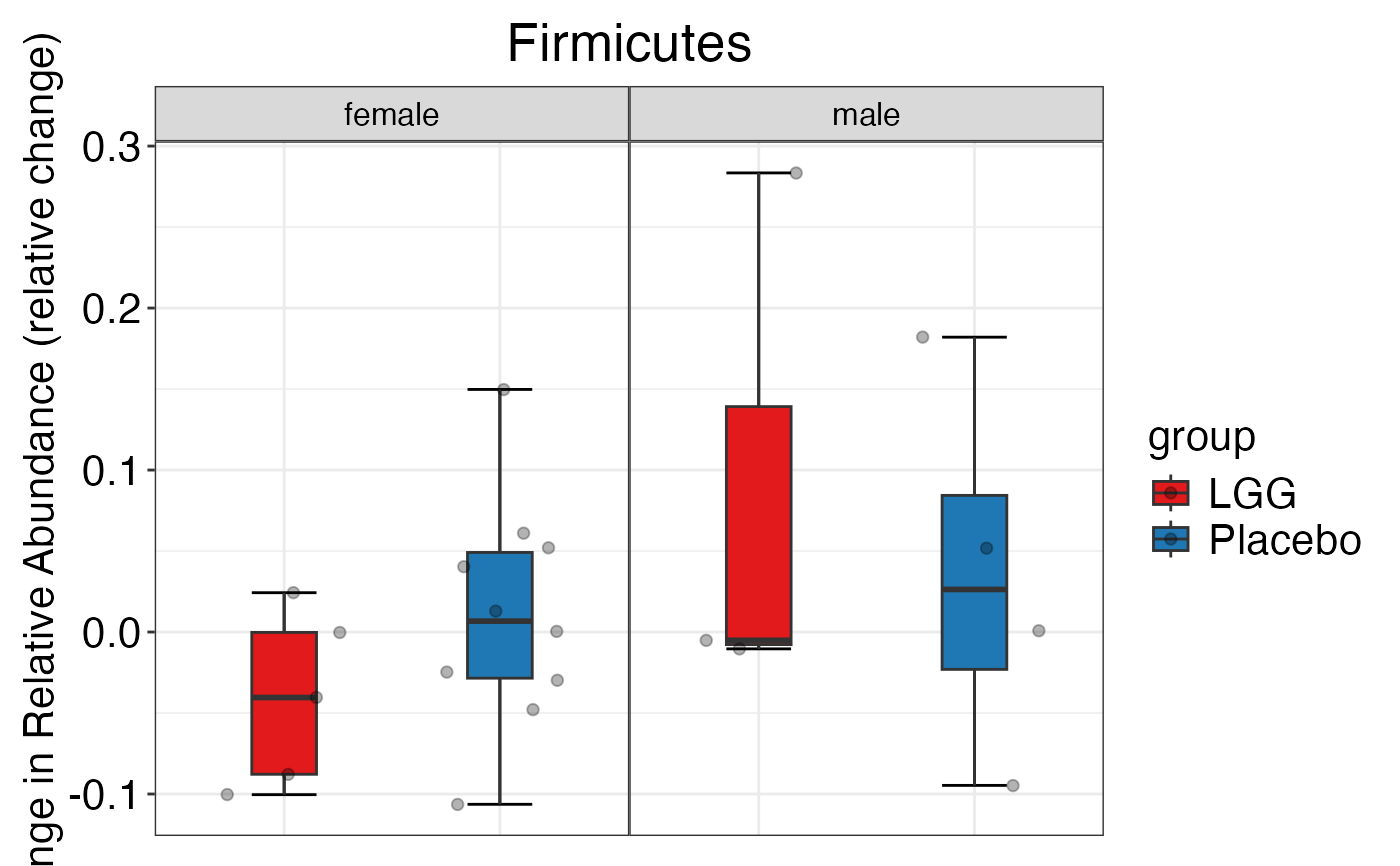
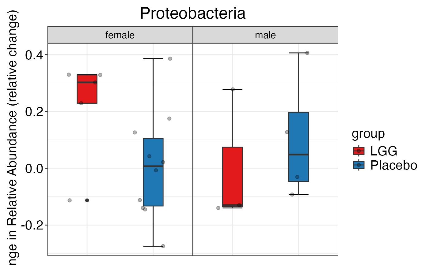
#> $Phylum
#> $Phylum$Phylum
#> $Phylum$Phylum$average
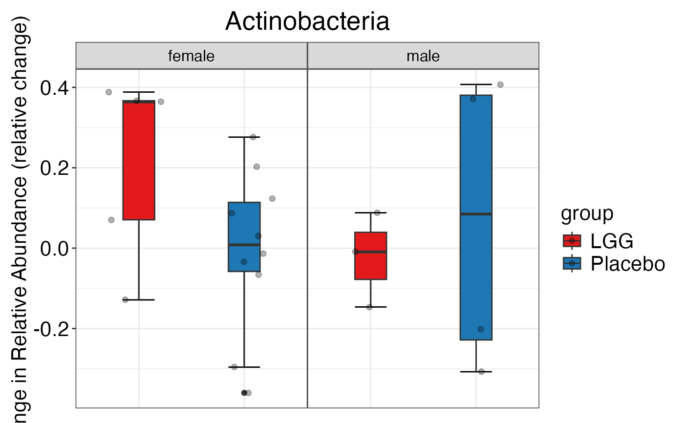 #>
#> $Phylum$Phylum$indiv
#>
#> $Phylum$Phylum$indiv
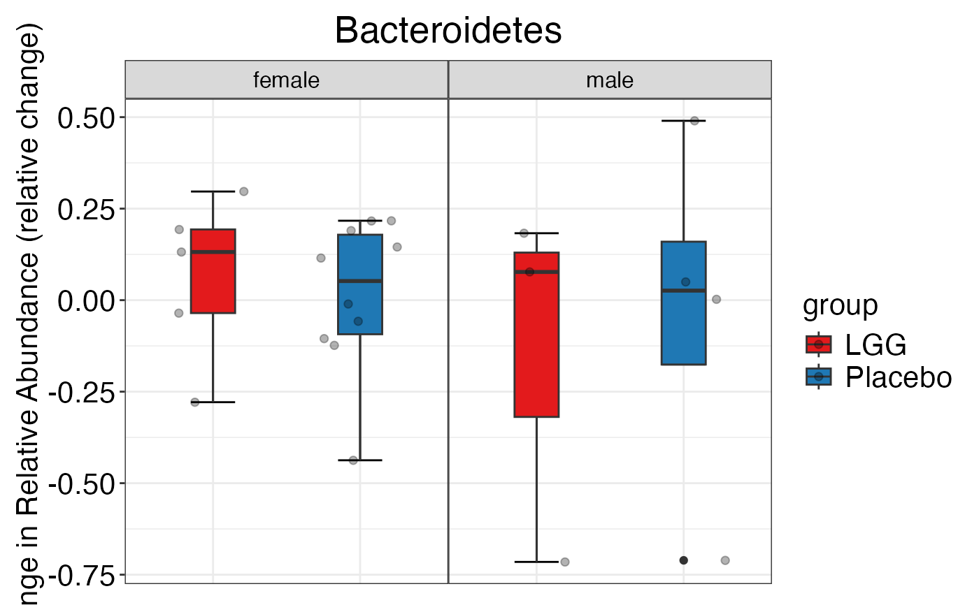 #>
#>
#>
#> $Family
#> $Family$Family
#> $Family$Family$average
#>
#>
#>
#> $Family
#> $Family$Family
#> $Family$Family$average
 #>
#> $Family$Family$indiv
#>
#> $Family$Family$indiv
 #>
#>
#>
#> $Genus
#> $Genus$Genus
#> $Genus$Genus$average
#>
#>
#>
#> $Genus
#> $Genus$Genus
#> $Genus$Genus$average
 #>
#> $Genus$Genus$indiv
#>
#> $Genus$Genus$indiv
 #>
#>
#>
plot_feature_diversity(
data.obj = peerj32.obj,
group.var = "group",
strata.var = "sex",
subject.var = "subject",
time.var = "time",
time.point.plot = c("1", "2"),
is.plot.change = FALSE,
feature.change.func = "relative change",
feature.level = c("Phylum", "Family", "Genus"),
prop.to.lump = 0.0001,
top.k.plot = NULL,
top.k.func = NULL,
renormalize = FALSE,
plot.other = TRUE,
plot.scheme = 'combined',
plot.type = "heatmap"
)
#> Validation passed.
#> Your data is in raw format ('Raw'). Normalization is crucial for further analyses. Now, 'mStat_normalize_data' function is automatically applying 'TSS' transformation.
#> Data has been successfully normalized using TSS method.
#> Validation passed.
#> Your data is in raw format ('Raw'). Normalization is crucial for further analyses. Now, 'mStat_normalize_data' function is automatically applying 'TSS' transformation.
#> Data has been successfully normalized using TSS method.
#> Validation passed.
#> Your data is in raw format ('Raw'). Normalization is crucial for further analyses. Now, 'mStat_normalize_data' function is automatically applying 'TSS' transformation.
#> Data has been successfully normalized using TSS method.
#> $Phylum
#> $Phylum$Phylum
#> $Phylum$Phylum$indiv
#>
#>
#>
plot_feature_diversity(
data.obj = peerj32.obj,
group.var = "group",
strata.var = "sex",
subject.var = "subject",
time.var = "time",
time.point.plot = c("1", "2"),
is.plot.change = FALSE,
feature.change.func = "relative change",
feature.level = c("Phylum", "Family", "Genus"),
prop.to.lump = 0.0001,
top.k.plot = NULL,
top.k.func = NULL,
renormalize = FALSE,
plot.other = TRUE,
plot.scheme = 'combined',
plot.type = "heatmap"
)
#> Validation passed.
#> Your data is in raw format ('Raw'). Normalization is crucial for further analyses. Now, 'mStat_normalize_data' function is automatically applying 'TSS' transformation.
#> Data has been successfully normalized using TSS method.
#> Validation passed.
#> Your data is in raw format ('Raw'). Normalization is crucial for further analyses. Now, 'mStat_normalize_data' function is automatically applying 'TSS' transformation.
#> Data has been successfully normalized using TSS method.
#> Validation passed.
#> Your data is in raw format ('Raw'). Normalization is crucial for further analyses. Now, 'mStat_normalize_data' function is automatically applying 'TSS' transformation.
#> Data has been successfully normalized using TSS method.
#> $Phylum
#> $Phylum$Phylum
#> $Phylum$Phylum$indiv
 #>
#> $Phylum$Phylum$average
#>
#> $Phylum$Phylum$average
 #>
#>
#>
#> $Family
#> $Family$Family
#> $Family$Family$indiv
#>
#>
#>
#> $Family
#> $Family$Family
#> $Family$Family$indiv
 #>
#> $Family$Family$average
#>
#> $Family$Family$average
 #>
#>
#>
#> $Genus
#> $Genus$Genus
#> $Genus$Genus$indiv
#>
#>
#>
#> $Genus
#> $Genus$Genus
#> $Genus$Genus$indiv
 #>
#> $Genus$Genus$average
#>
#> $Genus$Genus$average
 #>
#>
#>
plot_feature_diversity(
data.obj = peerj32.obj,
group.var = "group",
strata.var = "sex",
subject.var = "subject",
time.var = "time",
time.point.plot = c("1", "2"),
is.plot.change = FALSE,
feature.level = c("Phylum", "Family", "Genus"),
prop.to.lump = 0.0001,
top.k.plot = NULL,
top.k.func = NULL,
renormalize = FALSE,
plot.other = TRUE,
plot.scheme = 'individual',
plot.type = "boxplot"
)
#> Validation passed.
#> Your data is in raw format ('Raw'). Normalization is crucial for further analyses. Now, 'mStat_normalize_data' function is automatically applying 'TSS' transformation.
#> Data has been successfully normalized using TSS method.
#> Validation passed.
#> Your data is in raw format ('Raw'). Normalization is crucial for further analyses. Now, 'mStat_normalize_data' function is automatically applying 'TSS' transformation.
#> Data has been successfully normalized using TSS method.
#> Validation passed.
#> Your data is in raw format ('Raw'). Normalization is crucial for further analyses. Now, 'mStat_normalize_data' function is automatically applying 'TSS' transformation.
#> Data has been successfully normalized using TSS method.
#> $Phylum
#> $Phylum$Phylum
#> $Phylum$Phylum$Actinobacteria
#>
#>
#>
plot_feature_diversity(
data.obj = peerj32.obj,
group.var = "group",
strata.var = "sex",
subject.var = "subject",
time.var = "time",
time.point.plot = c("1", "2"),
is.plot.change = FALSE,
feature.level = c("Phylum", "Family", "Genus"),
prop.to.lump = 0.0001,
top.k.plot = NULL,
top.k.func = NULL,
renormalize = FALSE,
plot.other = TRUE,
plot.scheme = 'individual',
plot.type = "boxplot"
)
#> Validation passed.
#> Your data is in raw format ('Raw'). Normalization is crucial for further analyses. Now, 'mStat_normalize_data' function is automatically applying 'TSS' transformation.
#> Data has been successfully normalized using TSS method.
#> Validation passed.
#> Your data is in raw format ('Raw'). Normalization is crucial for further analyses. Now, 'mStat_normalize_data' function is automatically applying 'TSS' transformation.
#> Data has been successfully normalized using TSS method.
#> Validation passed.
#> Your data is in raw format ('Raw'). Normalization is crucial for further analyses. Now, 'mStat_normalize_data' function is automatically applying 'TSS' transformation.
#> Data has been successfully normalized using TSS method.
#> $Phylum
#> $Phylum$Phylum
#> $Phylum$Phylum$Actinobacteria
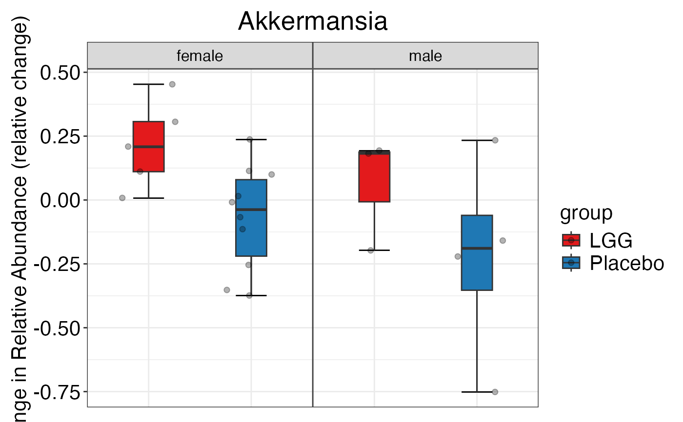 #>
#> $Phylum$Phylum$Bacteroidetes
#>
#> $Phylum$Phylum$Bacteroidetes
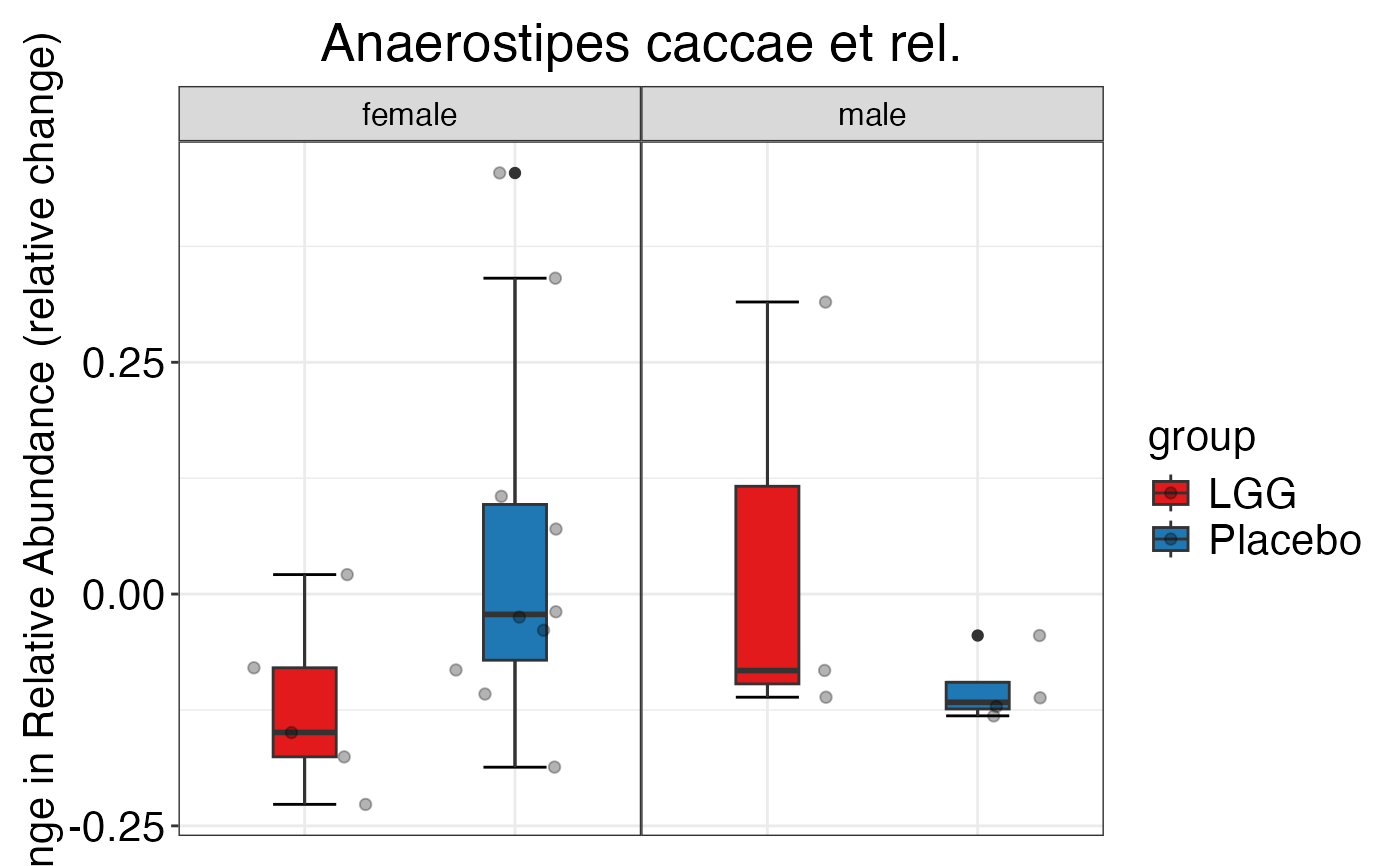 #>
#> $Phylum$Phylum$Firmicutes
#>
#> $Phylum$Phylum$Firmicutes
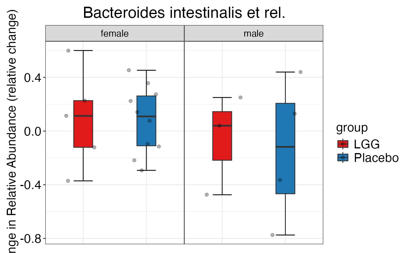 #>
#> $Phylum$Phylum$Proteobacteria
#>
#> $Phylum$Phylum$Proteobacteria
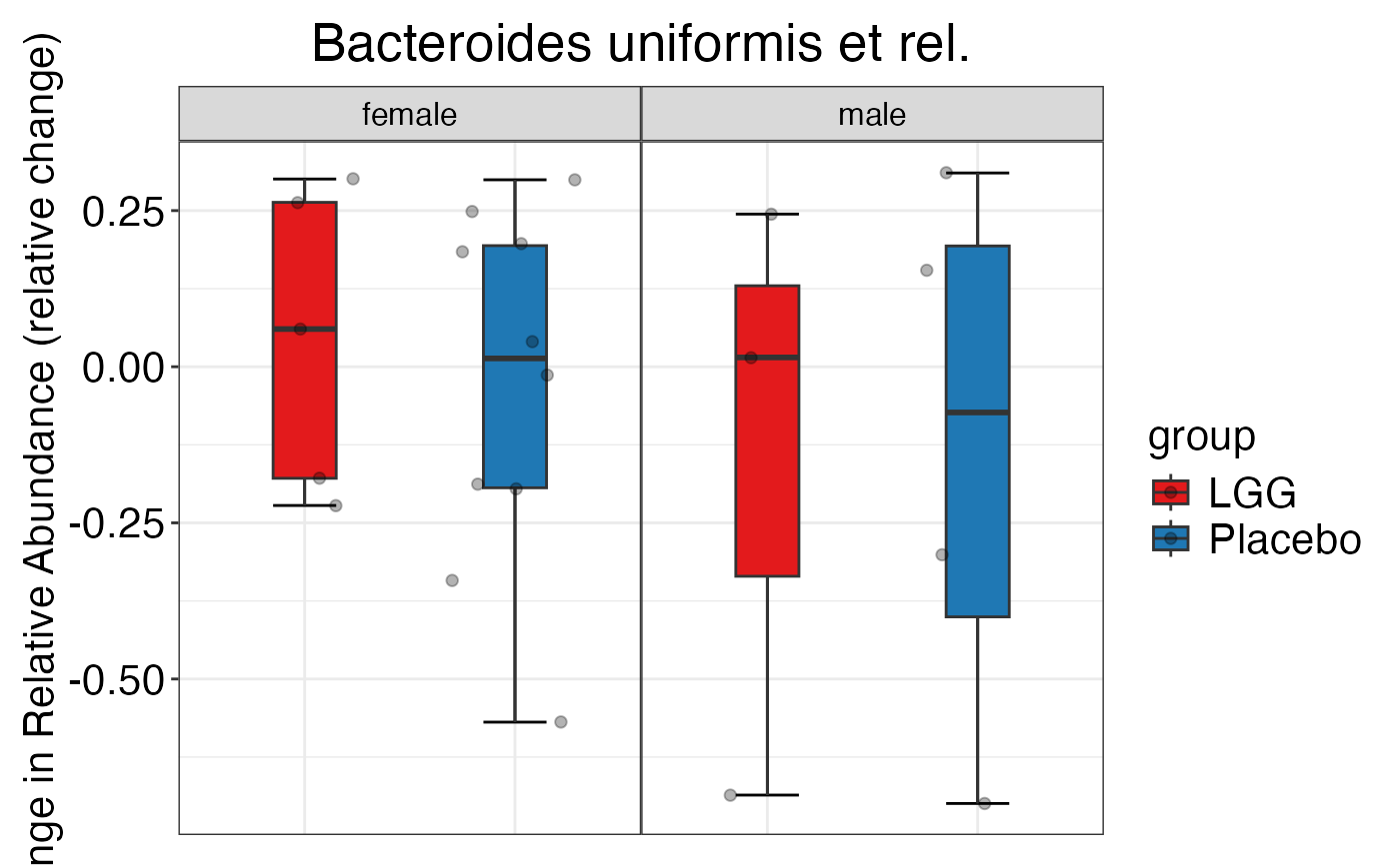 #>
#> $Phylum$Phylum$Verrucomicrobia
#>
#> $Phylum$Phylum$Verrucomicrobia
 #>
#>
#>
#> $Family
#> $Family$Family
#> $Family$Family$Actinobacteria
#>
#>
#>
#> $Family
#> $Family$Family
#> $Family$Family$Actinobacteria
 #>
#> $Family$Family$Bacilli
#>
#> $Family$Family$Bacilli
 #>
#> $Family$Family$Bacteroidetes
#>
#> $Family$Family$Bacteroidetes
 #>
#> $Family$Family$`Clostridium cluster IV`
#>
#> $Family$Family$`Clostridium cluster IV`
 #>
#> $Family$Family$`Clostridium cluster XIVa`
#>
#> $Family$Family$`Clostridium cluster XIVa`
 #>
#> $Family$Family$Proteobacteria
#>
#> $Family$Family$Proteobacteria
 #>
#>
#>
#> $Genus
#> $Genus$Genus
#> $Genus$Genus$Akkermansia
#>
#>
#>
#> $Genus
#> $Genus$Genus
#> $Genus$Genus$Akkermansia
 #>
#> $Genus$Genus$`Anaerostipes caccae et rel.`
#>
#> $Genus$Genus$`Anaerostipes caccae et rel.`
 #>
#> $Genus$Genus$`Bacteroides intestinalis et rel.`
#>
#> $Genus$Genus$`Bacteroides intestinalis et rel.`
 #>
#> $Genus$Genus$`Bacteroides uniformis et rel.`
#>
#> $Genus$Genus$`Bacteroides uniformis et rel.`
 #>
#> $Genus$Genus$`Bacteroides vulgatus et rel.`
#>
#> $Genus$Genus$`Bacteroides vulgatus et rel.`
 #>
#> $Genus$Genus$Bifidobacterium
#>
#> $Genus$Genus$Bifidobacterium
 #>
#>
#>
plot_feature_diversity(
data.obj = peerj32.obj,
group.var = "group",
strata.var = "sex",
subject.var = "subject",
time.var = "time",
time.point.plot = c("1", "2"),
is.plot.change = FALSE,
feature.level = c("Phylum", "Family", "Genus"),
prop.to.lump = 0.0001,
top.k.plot = NULL,
top.k.func = NULL,
renormalize = FALSE,
plot.other = TRUE,
plot.scheme = 'combined',
plot.type = "barplot"
)
#> Validation passed.
#> Your data is in raw count format. For barplot visualization, normalization is not required as ggplot2's position='fill' will automatically convert to proportions.
#> Warning: Removed 77 rows containing missing values or values outside the scale range
#> (`geom_segment()`).
#> Warning: Removed 35 rows containing missing values or values outside the scale range
#> (`geom_segment()`).
#> Warning: Removed 28 rows containing missing values or values outside the scale range
#> (`geom_segment()`).
#> Warning: Removed 21 rows containing missing values or values outside the scale range
#> (`geom_segment()`).
#> Warning: Removed 7 rows containing missing values or values outside the scale range
#> (`geom_segment()`).
#> Warning: Removed 7 rows containing missing values or values outside the scale range
#> (`geom_segment()`).
#> Warning: Removed 7 rows containing missing values or values outside the scale range
#> (`geom_segment()`).
#> Warning: Removed 7 rows containing missing values or values outside the scale range
#> (`geom_segment()`).
#> Validation passed.
#> Your data is in raw count format. For barplot visualization, normalization is not required as ggplot2's position='fill' will automatically convert to proportions.
#> Warning: Removed 209 rows containing missing values or values outside the scale range
#> (`geom_segment()`).
#> Warning: Removed 95 rows containing missing values or values outside the scale range
#> (`geom_segment()`).
#> Warning: Removed 76 rows containing missing values or values outside the scale range
#> (`geom_segment()`).
#> Warning: Removed 57 rows containing missing values or values outside the scale range
#> (`geom_segment()`).
#> Warning: Removed 19 rows containing missing values or values outside the scale range
#> (`geom_segment()`).
#> Warning: Removed 19 rows containing missing values or values outside the scale range
#> (`geom_segment()`).
#> Warning: Removed 19 rows containing missing values or values outside the scale range
#> (`geom_segment()`).
#> Warning: Removed 19 rows containing missing values or values outside the scale range
#> (`geom_segment()`).
#> Validation passed.
#> Your data is in raw count format. For barplot visualization, normalization is not required as ggplot2's position='fill' will automatically convert to proportions.
#> Warning: Removed 231 rows containing missing values or values outside the scale range
#> (`geom_segment()`).
#> Warning: Removed 105 rows containing missing values or values outside the scale range
#> (`geom_segment()`).
#> Warning: Removed 84 rows containing missing values or values outside the scale range
#> (`geom_segment()`).
#> Warning: Removed 63 rows containing missing values or values outside the scale range
#> (`geom_segment()`).
#> Warning: Removed 21 rows containing missing values or values outside the scale range
#> (`geom_segment()`).
#> Warning: Removed 21 rows containing missing values or values outside the scale range
#> (`geom_segment()`).
#> Warning: Removed 21 rows containing missing values or values outside the scale range
#> (`geom_segment()`).
#> Warning: Removed 21 rows containing missing values or values outside the scale range
#> (`geom_segment()`).
#> $Phylum
#> $Phylum$Phylum
#> $Phylum$Phylum$indiv
#> Warning: Removed 77 rows containing missing values or values outside the scale range
#> (`geom_segment()`).
#> Warning: Removed 35 rows containing missing values or values outside the scale range
#> (`geom_segment()`).
#> Warning: Removed 28 rows containing missing values or values outside the scale range
#> (`geom_segment()`).
#> Warning: Removed 21 rows containing missing values or values outside the scale range
#> (`geom_segment()`).
#>
#>
#>
plot_feature_diversity(
data.obj = peerj32.obj,
group.var = "group",
strata.var = "sex",
subject.var = "subject",
time.var = "time",
time.point.plot = c("1", "2"),
is.plot.change = FALSE,
feature.level = c("Phylum", "Family", "Genus"),
prop.to.lump = 0.0001,
top.k.plot = NULL,
top.k.func = NULL,
renormalize = FALSE,
plot.other = TRUE,
plot.scheme = 'combined',
plot.type = "barplot"
)
#> Validation passed.
#> Your data is in raw count format. For barplot visualization, normalization is not required as ggplot2's position='fill' will automatically convert to proportions.
#> Warning: Removed 77 rows containing missing values or values outside the scale range
#> (`geom_segment()`).
#> Warning: Removed 35 rows containing missing values or values outside the scale range
#> (`geom_segment()`).
#> Warning: Removed 28 rows containing missing values or values outside the scale range
#> (`geom_segment()`).
#> Warning: Removed 21 rows containing missing values or values outside the scale range
#> (`geom_segment()`).
#> Warning: Removed 7 rows containing missing values or values outside the scale range
#> (`geom_segment()`).
#> Warning: Removed 7 rows containing missing values or values outside the scale range
#> (`geom_segment()`).
#> Warning: Removed 7 rows containing missing values or values outside the scale range
#> (`geom_segment()`).
#> Warning: Removed 7 rows containing missing values or values outside the scale range
#> (`geom_segment()`).
#> Validation passed.
#> Your data is in raw count format. For barplot visualization, normalization is not required as ggplot2's position='fill' will automatically convert to proportions.
#> Warning: Removed 209 rows containing missing values or values outside the scale range
#> (`geom_segment()`).
#> Warning: Removed 95 rows containing missing values or values outside the scale range
#> (`geom_segment()`).
#> Warning: Removed 76 rows containing missing values or values outside the scale range
#> (`geom_segment()`).
#> Warning: Removed 57 rows containing missing values or values outside the scale range
#> (`geom_segment()`).
#> Warning: Removed 19 rows containing missing values or values outside the scale range
#> (`geom_segment()`).
#> Warning: Removed 19 rows containing missing values or values outside the scale range
#> (`geom_segment()`).
#> Warning: Removed 19 rows containing missing values or values outside the scale range
#> (`geom_segment()`).
#> Warning: Removed 19 rows containing missing values or values outside the scale range
#> (`geom_segment()`).
#> Validation passed.
#> Your data is in raw count format. For barplot visualization, normalization is not required as ggplot2's position='fill' will automatically convert to proportions.
#> Warning: Removed 231 rows containing missing values or values outside the scale range
#> (`geom_segment()`).
#> Warning: Removed 105 rows containing missing values or values outside the scale range
#> (`geom_segment()`).
#> Warning: Removed 84 rows containing missing values or values outside the scale range
#> (`geom_segment()`).
#> Warning: Removed 63 rows containing missing values or values outside the scale range
#> (`geom_segment()`).
#> Warning: Removed 21 rows containing missing values or values outside the scale range
#> (`geom_segment()`).
#> Warning: Removed 21 rows containing missing values or values outside the scale range
#> (`geom_segment()`).
#> Warning: Removed 21 rows containing missing values or values outside the scale range
#> (`geom_segment()`).
#> Warning: Removed 21 rows containing missing values or values outside the scale range
#> (`geom_segment()`).
#> $Phylum
#> $Phylum$Phylum
#> $Phylum$Phylum$indiv
#> Warning: Removed 77 rows containing missing values or values outside the scale range
#> (`geom_segment()`).
#> Warning: Removed 35 rows containing missing values or values outside the scale range
#> (`geom_segment()`).
#> Warning: Removed 28 rows containing missing values or values outside the scale range
#> (`geom_segment()`).
#> Warning: Removed 21 rows containing missing values or values outside the scale range
#> (`geom_segment()`).
 #>
#> $Phylum$Phylum$average
#> Warning: Removed 7 rows containing missing values or values outside the scale range
#> (`geom_segment()`).
#> Warning: Removed 7 rows containing missing values or values outside the scale range
#> (`geom_segment()`).
#> Warning: Removed 7 rows containing missing values or values outside the scale range
#> (`geom_segment()`).
#> Warning: Removed 7 rows containing missing values or values outside the scale range
#> (`geom_segment()`).
#>
#> $Phylum$Phylum$average
#> Warning: Removed 7 rows containing missing values or values outside the scale range
#> (`geom_segment()`).
#> Warning: Removed 7 rows containing missing values or values outside the scale range
#> (`geom_segment()`).
#> Warning: Removed 7 rows containing missing values or values outside the scale range
#> (`geom_segment()`).
#> Warning: Removed 7 rows containing missing values or values outside the scale range
#> (`geom_segment()`).
 #>
#>
#>
#> $Family
#> $Family$Family
#> $Family$Family$indiv
#> Warning: Removed 209 rows containing missing values or values outside the scale range
#> (`geom_segment()`).
#> Warning: Removed 95 rows containing missing values or values outside the scale range
#> (`geom_segment()`).
#> Warning: Removed 76 rows containing missing values or values outside the scale range
#> (`geom_segment()`).
#> Warning: Removed 57 rows containing missing values or values outside the scale range
#> (`geom_segment()`).
#>
#>
#>
#> $Family
#> $Family$Family
#> $Family$Family$indiv
#> Warning: Removed 209 rows containing missing values or values outside the scale range
#> (`geom_segment()`).
#> Warning: Removed 95 rows containing missing values or values outside the scale range
#> (`geom_segment()`).
#> Warning: Removed 76 rows containing missing values or values outside the scale range
#> (`geom_segment()`).
#> Warning: Removed 57 rows containing missing values or values outside the scale range
#> (`geom_segment()`).
 #>
#> $Family$Family$average
#> Warning: Removed 19 rows containing missing values or values outside the scale range
#> (`geom_segment()`).
#> Warning: Removed 19 rows containing missing values or values outside the scale range
#> (`geom_segment()`).
#> Warning: Removed 19 rows containing missing values or values outside the scale range
#> (`geom_segment()`).
#> Warning: Removed 19 rows containing missing values or values outside the scale range
#> (`geom_segment()`).
#>
#> $Family$Family$average
#> Warning: Removed 19 rows containing missing values or values outside the scale range
#> (`geom_segment()`).
#> Warning: Removed 19 rows containing missing values or values outside the scale range
#> (`geom_segment()`).
#> Warning: Removed 19 rows containing missing values or values outside the scale range
#> (`geom_segment()`).
#> Warning: Removed 19 rows containing missing values or values outside the scale range
#> (`geom_segment()`).
 #>
#>
#>
#> $Genus
#> $Genus$Genus
#> $Genus$Genus$indiv
#> Warning: Removed 231 rows containing missing values or values outside the scale range
#> (`geom_segment()`).
#> Warning: Removed 105 rows containing missing values or values outside the scale range
#> (`geom_segment()`).
#> Warning: Removed 84 rows containing missing values or values outside the scale range
#> (`geom_segment()`).
#> Warning: Removed 63 rows containing missing values or values outside the scale range
#> (`geom_segment()`).
#>
#>
#>
#> $Genus
#> $Genus$Genus
#> $Genus$Genus$indiv
#> Warning: Removed 231 rows containing missing values or values outside the scale range
#> (`geom_segment()`).
#> Warning: Removed 105 rows containing missing values or values outside the scale range
#> (`geom_segment()`).
#> Warning: Removed 84 rows containing missing values or values outside the scale range
#> (`geom_segment()`).
#> Warning: Removed 63 rows containing missing values or values outside the scale range
#> (`geom_segment()`).
 #>
#> $Genus$Genus$average
#> Warning: Removed 21 rows containing missing values or values outside the scale range
#> (`geom_segment()`).
#> Warning: Removed 21 rows containing missing values or values outside the scale range
#> (`geom_segment()`).
#> Warning: Removed 21 rows containing missing values or values outside the scale range
#> (`geom_segment()`).
#> Warning: Removed 21 rows containing missing values or values outside the scale range
#> (`geom_segment()`).
#>
#> $Genus$Genus$average
#> Warning: Removed 21 rows containing missing values or values outside the scale range
#> (`geom_segment()`).
#> Warning: Removed 21 rows containing missing values or values outside the scale range
#> (`geom_segment()`).
#> Warning: Removed 21 rows containing missing values or values outside the scale range
#> (`geom_segment()`).
#> Warning: Removed 21 rows containing missing values or values outside the scale range
#> (`geom_segment()`).
 #>
#>
#>
plot_feature_diversity(
data.obj = peerj32.obj,
group.var = "group",
strata.var = "sex",
subject.var = "subject",
time.var = "time",
time.point.plot = c("1", "2"),
is.plot.change = FALSE,
feature.level = c("Family"),
features.plot = unique(peerj32.obj$feature.ann[, "Family"])[11:20],
prop.to.lump = 0.0001,
top.k.plot = NULL,
top.k.func = NULL,
renormalize = FALSE,
plot.other = TRUE,
plot.scheme = 'combined',
plot.type = "barplot"
)
#> Validation passed.
#> Your data is in raw count format. For barplot visualization, normalization is not required as ggplot2's position='fill' will automatically convert to proportions.
#> Warning: Removed 110 rows containing missing values or values outside the scale range
#> (`geom_segment()`).
#> Warning: Removed 50 rows containing missing values or values outside the scale range
#> (`geom_segment()`).
#> Warning: Removed 40 rows containing missing values or values outside the scale range
#> (`geom_segment()`).
#> Warning: Removed 30 rows containing missing values or values outside the scale range
#> (`geom_segment()`).
#> Warning: Removed 10 rows containing missing values or values outside the scale range
#> (`geom_segment()`).
#> Warning: Removed 10 rows containing missing values or values outside the scale range
#> (`geom_segment()`).
#> Warning: Removed 10 rows containing missing values or values outside the scale range
#> (`geom_segment()`).
#> Warning: Removed 10 rows containing missing values or values outside the scale range
#> (`geom_segment()`).
#> $Family
#> $Family$Family
#> $Family$Family$indiv
#> Warning: Removed 110 rows containing missing values or values outside the scale range
#> (`geom_segment()`).
#> Warning: Removed 50 rows containing missing values or values outside the scale range
#> (`geom_segment()`).
#> Warning: Removed 40 rows containing missing values or values outside the scale range
#> (`geom_segment()`).
#> Warning: Removed 30 rows containing missing values or values outside the scale range
#> (`geom_segment()`).
#>
#>
#>
plot_feature_diversity(
data.obj = peerj32.obj,
group.var = "group",
strata.var = "sex",
subject.var = "subject",
time.var = "time",
time.point.plot = c("1", "2"),
is.plot.change = FALSE,
feature.level = c("Family"),
features.plot = unique(peerj32.obj$feature.ann[, "Family"])[11:20],
prop.to.lump = 0.0001,
top.k.plot = NULL,
top.k.func = NULL,
renormalize = FALSE,
plot.other = TRUE,
plot.scheme = 'combined',
plot.type = "barplot"
)
#> Validation passed.
#> Your data is in raw count format. For barplot visualization, normalization is not required as ggplot2's position='fill' will automatically convert to proportions.
#> Warning: Removed 110 rows containing missing values or values outside the scale range
#> (`geom_segment()`).
#> Warning: Removed 50 rows containing missing values or values outside the scale range
#> (`geom_segment()`).
#> Warning: Removed 40 rows containing missing values or values outside the scale range
#> (`geom_segment()`).
#> Warning: Removed 30 rows containing missing values or values outside the scale range
#> (`geom_segment()`).
#> Warning: Removed 10 rows containing missing values or values outside the scale range
#> (`geom_segment()`).
#> Warning: Removed 10 rows containing missing values or values outside the scale range
#> (`geom_segment()`).
#> Warning: Removed 10 rows containing missing values or values outside the scale range
#> (`geom_segment()`).
#> Warning: Removed 10 rows containing missing values or values outside the scale range
#> (`geom_segment()`).
#> $Family
#> $Family$Family
#> $Family$Family$indiv
#> Warning: Removed 110 rows containing missing values or values outside the scale range
#> (`geom_segment()`).
#> Warning: Removed 50 rows containing missing values or values outside the scale range
#> (`geom_segment()`).
#> Warning: Removed 40 rows containing missing values or values outside the scale range
#> (`geom_segment()`).
#> Warning: Removed 30 rows containing missing values or values outside the scale range
#> (`geom_segment()`).
 #>
#> $Family$Family$average
#> Warning: Removed 10 rows containing missing values or values outside the scale range
#> (`geom_segment()`).
#> Warning: Removed 10 rows containing missing values or values outside the scale range
#> (`geom_segment()`).
#> Warning: Removed 10 rows containing missing values or values outside the scale range
#> (`geom_segment()`).
#> Warning: Removed 10 rows containing missing values or values outside the scale range
#> (`geom_segment()`).
#>
#> $Family$Family$average
#> Warning: Removed 10 rows containing missing values or values outside the scale range
#> (`geom_segment()`).
#> Warning: Removed 10 rows containing missing values or values outside the scale range
#> (`geom_segment()`).
#> Warning: Removed 10 rows containing missing values or values outside the scale range
#> (`geom_segment()`).
#> Warning: Removed 10 rows containing missing values or values outside the scale range
#> (`geom_segment()`).
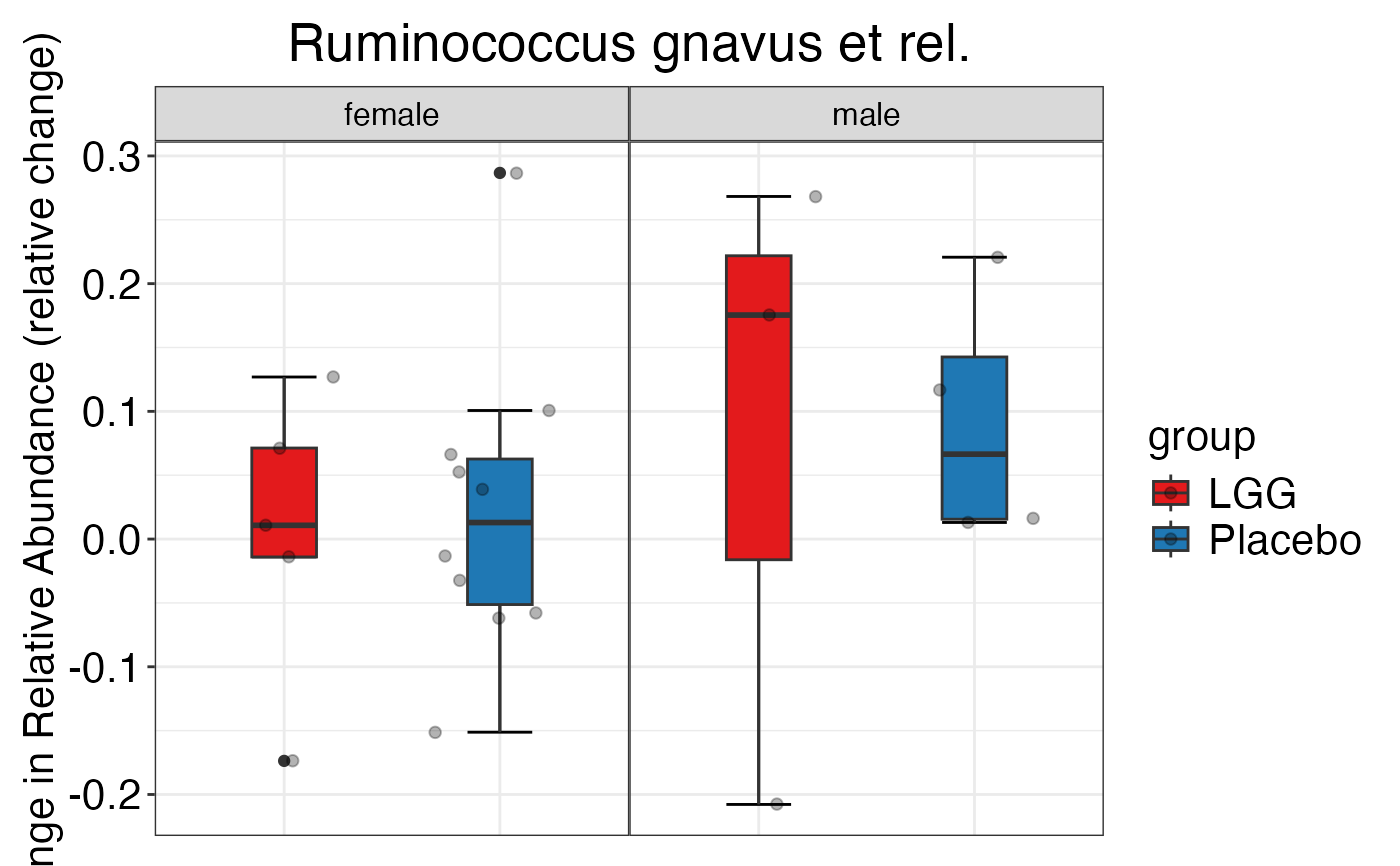 #>
#>
#>
plot_feature_diversity(
data.obj = peerj32.obj,
group.var = "group",
strata.var = "sex",
subject.var = "subject",
time.var = "time",
time.point.plot = c("1", "2"),
is.plot.change = FALSE,
feature.level = c("Family"),
prop.to.lump = 0.0001,
top.k.plot = NULL,
top.k.func = NULL,
renormalize = FALSE,
plot.other = TRUE,
plot.scheme = 'combined',
plot.type = "dotplot"
)
#> Validation passed.
#> Your data is in raw format ('Raw'). Normalization is crucial for further analyses. Now, 'mStat_normalize_data' function is automatically applying 'TSS' transformation.
#> Data has been successfully normalized using TSS method.
#> $Family
#> $Family$Family
#>
#>
#>
plot_feature_diversity(
data.obj = peerj32.obj,
group.var = "group",
strata.var = "sex",
subject.var = "subject",
time.var = "time",
time.point.plot = c("1", "2"),
is.plot.change = FALSE,
feature.level = c("Family"),
prop.to.lump = 0.0001,
top.k.plot = NULL,
top.k.func = NULL,
renormalize = FALSE,
plot.other = TRUE,
plot.scheme = 'combined',
plot.type = "dotplot"
)
#> Validation passed.
#> Your data is in raw format ('Raw'). Normalization is crucial for further analyses. Now, 'mStat_normalize_data' function is automatically applying 'TSS' transformation.
#> Data has been successfully normalized using TSS method.
#> $Family
#> $Family$Family
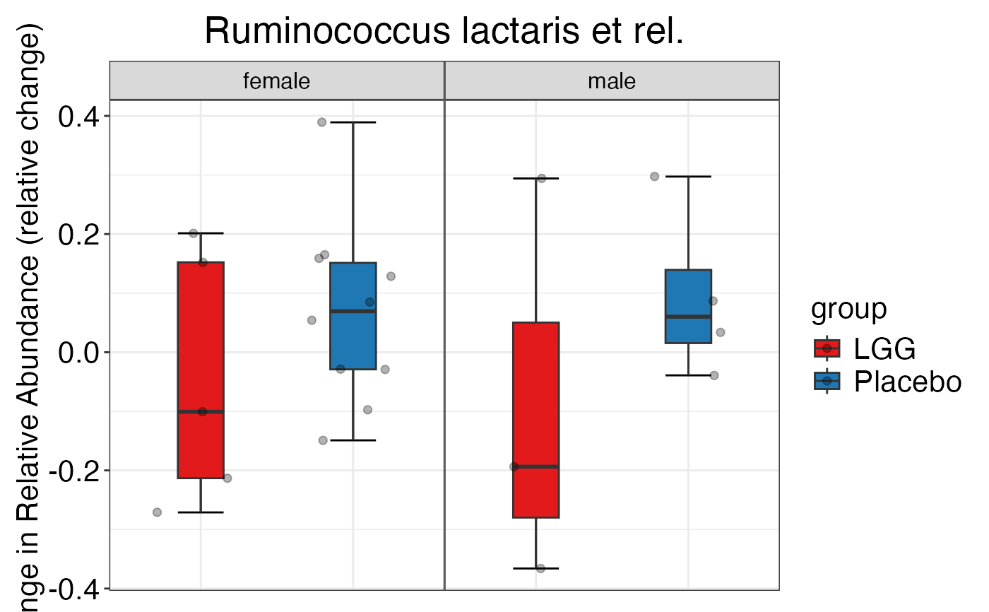 #>
#>
data(subset_T2D.obj)
plot_feature_diversity(
data.obj = subset_T2D.obj,
group.var = "sample_body_site",
strata.var = "subject_race",
subject.var = "subject_id",
time.var = "visit_number_num",
time.point.plot = unique(subset_T2D.obj$meta.dat$visit_number_num),
is.plot.change = FALSE,
feature.level = c("Family"),
prop.to.lump = 0.0001,
top.k.plot = NULL,
top.k.func = NULL,
renormalize = FALSE,
plot.other = TRUE,
plot.scheme = 'combined',
plot.type = "barplot"
)
#> Validation passed.
#> Your data is in raw count format. For barplot visualization, normalization is not required as ggplot2's position='fill' will automatically convert to proportions.
#> Warning: Removed 20 rows containing missing values or values outside the scale range
#> (`geom_segment()`).
#> Warning: Removed 20 rows containing missing values or values outside the scale range
#> (`geom_segment()`).
#> Warning: Removed 20 rows containing missing values or values outside the scale range
#> (`geom_segment()`).
#> Warning: Removed 20 rows containing missing values or values outside the scale range
#> (`geom_segment()`).
#> Warning: Removed 20 rows containing missing values or values outside the scale range
#> (`geom_segment()`).
#> Warning: Removed 20 rows containing missing values or values outside the scale range
#> (`geom_segment()`).
#> $Family
#> $Family$Family
#> Warning: Removed 20 rows containing missing values or values outside the scale range
#> (`geom_segment()`).
#> Warning: Removed 20 rows containing missing values or values outside the scale range
#> (`geom_segment()`).
#> Warning: Removed 20 rows containing missing values or values outside the scale range
#> (`geom_segment()`).
#> Warning: Removed 20 rows containing missing values or values outside the scale range
#> (`geom_segment()`).
#> Warning: Removed 20 rows containing missing values or values outside the scale range
#> (`geom_segment()`).
#> Warning: Removed 20 rows containing missing values or values outside the scale range
#> (`geom_segment()`).
#>
#>
data(subset_T2D.obj)
plot_feature_diversity(
data.obj = subset_T2D.obj,
group.var = "sample_body_site",
strata.var = "subject_race",
subject.var = "subject_id",
time.var = "visit_number_num",
time.point.plot = unique(subset_T2D.obj$meta.dat$visit_number_num),
is.plot.change = FALSE,
feature.level = c("Family"),
prop.to.lump = 0.0001,
top.k.plot = NULL,
top.k.func = NULL,
renormalize = FALSE,
plot.other = TRUE,
plot.scheme = 'combined',
plot.type = "barplot"
)
#> Validation passed.
#> Your data is in raw count format. For barplot visualization, normalization is not required as ggplot2's position='fill' will automatically convert to proportions.
#> Warning: Removed 20 rows containing missing values or values outside the scale range
#> (`geom_segment()`).
#> Warning: Removed 20 rows containing missing values or values outside the scale range
#> (`geom_segment()`).
#> Warning: Removed 20 rows containing missing values or values outside the scale range
#> (`geom_segment()`).
#> Warning: Removed 20 rows containing missing values or values outside the scale range
#> (`geom_segment()`).
#> Warning: Removed 20 rows containing missing values or values outside the scale range
#> (`geom_segment()`).
#> Warning: Removed 20 rows containing missing values or values outside the scale range
#> (`geom_segment()`).
#> $Family
#> $Family$Family
#> Warning: Removed 20 rows containing missing values or values outside the scale range
#> (`geom_segment()`).
#> Warning: Removed 20 rows containing missing values or values outside the scale range
#> (`geom_segment()`).
#> Warning: Removed 20 rows containing missing values or values outside the scale range
#> (`geom_segment()`).
#> Warning: Removed 20 rows containing missing values or values outside the scale range
#> (`geom_segment()`).
#> Warning: Removed 20 rows containing missing values or values outside the scale range
#> (`geom_segment()`).
#> Warning: Removed 20 rows containing missing values or values outside the scale range
#> (`geom_segment()`).
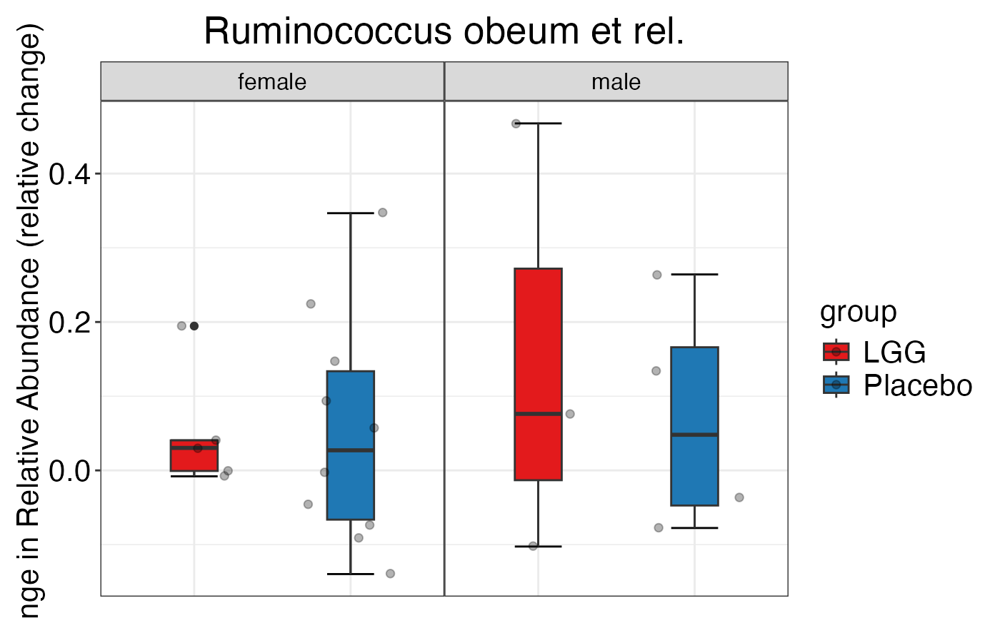 #>
#>
plot_feature_diversity(
data.obj = subset_T2D.obj,
group.var = "sample_body_site",
strata.var = "subject_race",
subject.var = "subject_id",
time.var = "visit_number_num",
time.point.plot = unique(subset_T2D.obj$meta.dat$visit_number_num),
is.plot.change = FALSE,
feature.level = c("Family"),
features.plot = unique(subset_T2D.obj$feature.ann[, "Family"])[1:10],
prop.to.lump = 0.0001,
top.k.plot = NULL,
top.k.func = NULL,
renormalize = FALSE,
plot.other = TRUE,
plot.scheme = 'combined',
plot.type = "barplot"
)
#> Validation passed.
#> Your data is in raw count format. For barplot visualization, normalization is not required as ggplot2's position='fill' will automatically convert to proportions.
#> Warning: Removed 9 rows containing missing values or values outside the scale range
#> (`geom_segment()`).
#> Warning: Removed 9 rows containing missing values or values outside the scale range
#> (`geom_segment()`).
#> Warning: Removed 9 rows containing missing values or values outside the scale range
#> (`geom_segment()`).
#> Warning: Removed 9 rows containing missing values or values outside the scale range
#> (`geom_segment()`).
#> Warning: Removed 9 rows containing missing values or values outside the scale range
#> (`geom_segment()`).
#> Warning: Removed 9 rows containing missing values or values outside the scale range
#> (`geom_segment()`).
#> $Family
#> $Family$Family
#> Warning: Removed 9 rows containing missing values or values outside the scale range
#> (`geom_segment()`).
#> Warning: Removed 9 rows containing missing values or values outside the scale range
#> (`geom_segment()`).
#> Warning: Removed 9 rows containing missing values or values outside the scale range
#> (`geom_segment()`).
#> Warning: Removed 9 rows containing missing values or values outside the scale range
#> (`geom_segment()`).
#> Warning: Removed 9 rows containing missing values or values outside the scale range
#> (`geom_segment()`).
#> Warning: Removed 9 rows containing missing values or values outside the scale range
#> (`geom_segment()`).
#>
#>
plot_feature_diversity(
data.obj = subset_T2D.obj,
group.var = "sample_body_site",
strata.var = "subject_race",
subject.var = "subject_id",
time.var = "visit_number_num",
time.point.plot = unique(subset_T2D.obj$meta.dat$visit_number_num),
is.plot.change = FALSE,
feature.level = c("Family"),
features.plot = unique(subset_T2D.obj$feature.ann[, "Family"])[1:10],
prop.to.lump = 0.0001,
top.k.plot = NULL,
top.k.func = NULL,
renormalize = FALSE,
plot.other = TRUE,
plot.scheme = 'combined',
plot.type = "barplot"
)
#> Validation passed.
#> Your data is in raw count format. For barplot visualization, normalization is not required as ggplot2's position='fill' will automatically convert to proportions.
#> Warning: Removed 9 rows containing missing values or values outside the scale range
#> (`geom_segment()`).
#> Warning: Removed 9 rows containing missing values or values outside the scale range
#> (`geom_segment()`).
#> Warning: Removed 9 rows containing missing values or values outside the scale range
#> (`geom_segment()`).
#> Warning: Removed 9 rows containing missing values or values outside the scale range
#> (`geom_segment()`).
#> Warning: Removed 9 rows containing missing values or values outside the scale range
#> (`geom_segment()`).
#> Warning: Removed 9 rows containing missing values or values outside the scale range
#> (`geom_segment()`).
#> $Family
#> $Family$Family
#> Warning: Removed 9 rows containing missing values or values outside the scale range
#> (`geom_segment()`).
#> Warning: Removed 9 rows containing missing values or values outside the scale range
#> (`geom_segment()`).
#> Warning: Removed 9 rows containing missing values or values outside the scale range
#> (`geom_segment()`).
#> Warning: Removed 9 rows containing missing values or values outside the scale range
#> (`geom_segment()`).
#> Warning: Removed 9 rows containing missing values or values outside the scale range
#> (`geom_segment()`).
#> Warning: Removed 9 rows containing missing values or values outside the scale range
#> (`geom_segment()`).
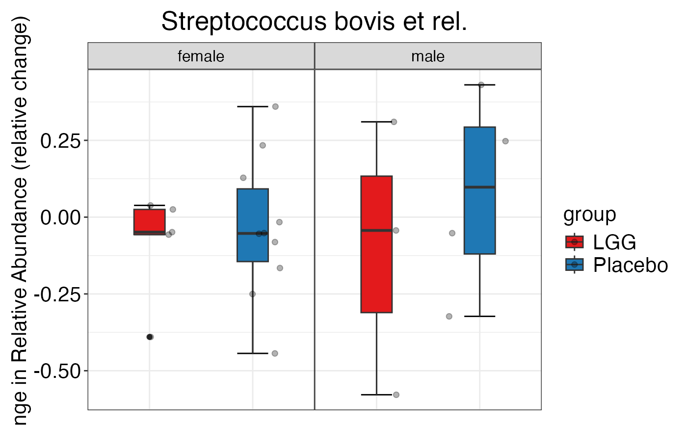 #>
#>
plot_feature_diversity(
data.obj = subset_T2D.obj,
group.var = "sample_body_site",
strata.var = "subject_race",
subject.var = "subject_id",
time.var = "visit_number_num",
time.point.plot = unique(subset_T2D.obj$meta.dat$visit_number_num),
features.plot = unique(subset_T2D.obj$feature.ann[, "Family"])[1:10],
is.plot.change = FALSE,
feature.level = c("Family"),
prop.to.lump = 0.0001,
top.k.plot = NULL,
top.k.func = NULL,
renormalize = FALSE,
plot.other = TRUE,
plot.scheme = 'combined',
plot.type = "areaplot"
)
#> Validation passed.
#> Your data is in raw format ('Raw'). Normalization is crucial for further analyses. Now, 'mStat_normalize_data' function is automatically applying 'TSS' transformation.
#> Data has been successfully normalized using TSS method.
#> Warning: No shared levels found between `names(values)` of the manual scale and the
#> data's colour values.
#> $Family
#> $Family$Family
#> Warning: No shared levels found between `names(values)` of the manual scale and the
#> data's colour values.
#>
#>
plot_feature_diversity(
data.obj = subset_T2D.obj,
group.var = "sample_body_site",
strata.var = "subject_race",
subject.var = "subject_id",
time.var = "visit_number_num",
time.point.plot = unique(subset_T2D.obj$meta.dat$visit_number_num),
features.plot = unique(subset_T2D.obj$feature.ann[, "Family"])[1:10],
is.plot.change = FALSE,
feature.level = c("Family"),
prop.to.lump = 0.0001,
top.k.plot = NULL,
top.k.func = NULL,
renormalize = FALSE,
plot.other = TRUE,
plot.scheme = 'combined',
plot.type = "areaplot"
)
#> Validation passed.
#> Your data is in raw format ('Raw'). Normalization is crucial for further analyses. Now, 'mStat_normalize_data' function is automatically applying 'TSS' transformation.
#> Data has been successfully normalized using TSS method.
#> Warning: No shared levels found between `names(values)` of the manual scale and the
#> data's colour values.
#> $Family
#> $Family$Family
#> Warning: No shared levels found between `names(values)` of the manual scale and the
#> data's colour values.
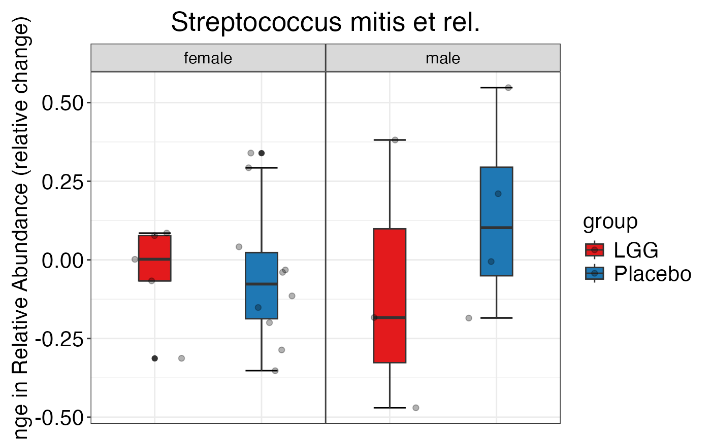 #>
#>
plot_feature_diversity(
data.obj = subset_T2D.obj,
group.var = "sample_body_site",
strata.var = "subject_race",
subject.var = "subject_id",
time.var = "visit_number_num",
time.point.plot = unique(subset_T2D.obj$meta.dat$visit_number_num),
is.plot.change = FALSE,
feature.level = c("Family"),
prop.to.lump = 0.0001,
top.k.plot = NULL,
top.k.func = NULL,
renormalize = FALSE,
plot.other = TRUE,
plot.scheme = 'combined',
plot.type = "spaghettiplot"
)
#> Validation passed.
#> Your data is in raw format ('Raw'). Normalization is crucial for further analyses. Now, 'mStat_normalize_data' function is automatically applying 'TSS' transformation.
#> Data has been successfully normalized using TSS method.
#> $Family
#> $Family$Family
#>
#>
plot_feature_diversity(
data.obj = subset_T2D.obj,
group.var = "sample_body_site",
strata.var = "subject_race",
subject.var = "subject_id",
time.var = "visit_number_num",
time.point.plot = unique(subset_T2D.obj$meta.dat$visit_number_num),
is.plot.change = FALSE,
feature.level = c("Family"),
prop.to.lump = 0.0001,
top.k.plot = NULL,
top.k.func = NULL,
renormalize = FALSE,
plot.other = TRUE,
plot.scheme = 'combined',
plot.type = "spaghettiplot"
)
#> Validation passed.
#> Your data is in raw format ('Raw'). Normalization is crucial for further analyses. Now, 'mStat_normalize_data' function is automatically applying 'TSS' transformation.
#> Data has been successfully normalized using TSS method.
#> $Family
#> $Family$Family
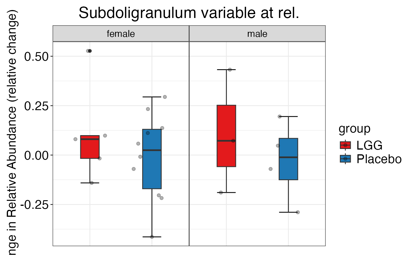 #>
#>
plot_feature_diversity(
data.obj = subset_T2D.obj,
group.var = "sample_body_site",
strata.var = "subject_race",
subject.var = "subject_id",
time.var = "visit_number_num",
time.point.plot = unique(subset_T2D.obj$meta.dat$visit_number_num),
is.plot.change = FALSE,
feature.level = c("Family"),
prop.to.lump = 0.0001,
top.k.plot = NULL,
top.k.func = NULL,
renormalize = FALSE,
plot.other = TRUE,
plot.scheme = 'individual',
plot.type = "spaghettiplot"
)
#> Validation passed.
#> Your data is in raw format ('Raw'). Normalization is crucial for further analyses. Now, 'mStat_normalize_data' function is automatically applying 'TSS' transformation.
#> Data has been successfully normalized using TSS method.
#> $Family
#> $Family$Family
#> $Family$Family$Aerococcaceae
#>
#>
plot_feature_diversity(
data.obj = subset_T2D.obj,
group.var = "sample_body_site",
strata.var = "subject_race",
subject.var = "subject_id",
time.var = "visit_number_num",
time.point.plot = unique(subset_T2D.obj$meta.dat$visit_number_num),
is.plot.change = FALSE,
feature.level = c("Family"),
prop.to.lump = 0.0001,
top.k.plot = NULL,
top.k.func = NULL,
renormalize = FALSE,
plot.other = TRUE,
plot.scheme = 'individual',
plot.type = "spaghettiplot"
)
#> Validation passed.
#> Your data is in raw format ('Raw'). Normalization is crucial for further analyses. Now, 'mStat_normalize_data' function is automatically applying 'TSS' transformation.
#> Data has been successfully normalized using TSS method.
#> $Family
#> $Family$Family
#> $Family$Family$Aerococcaceae
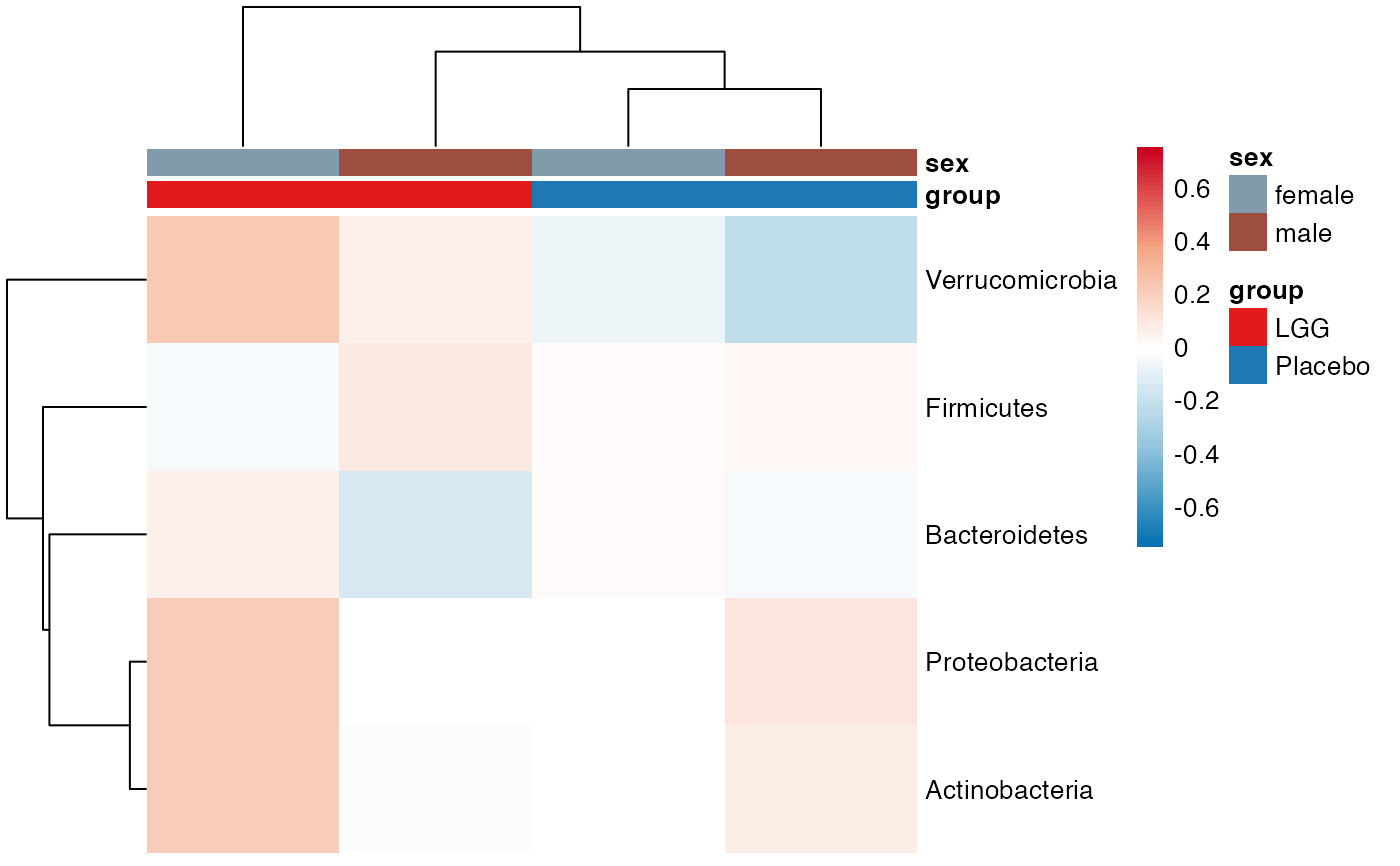 #>
#> $Family$Family$Bacteroidaceae
#>
#> $Family$Family$Bacteroidaceae
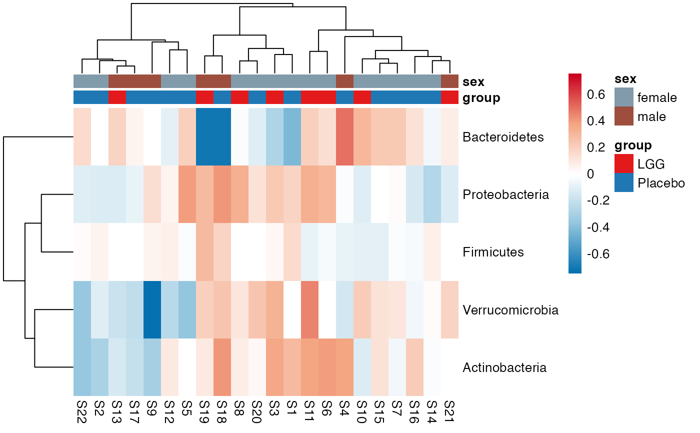 #>
#> $Family$Family$Corynebacteriaceae
#>
#> $Family$Family$Corynebacteriaceae
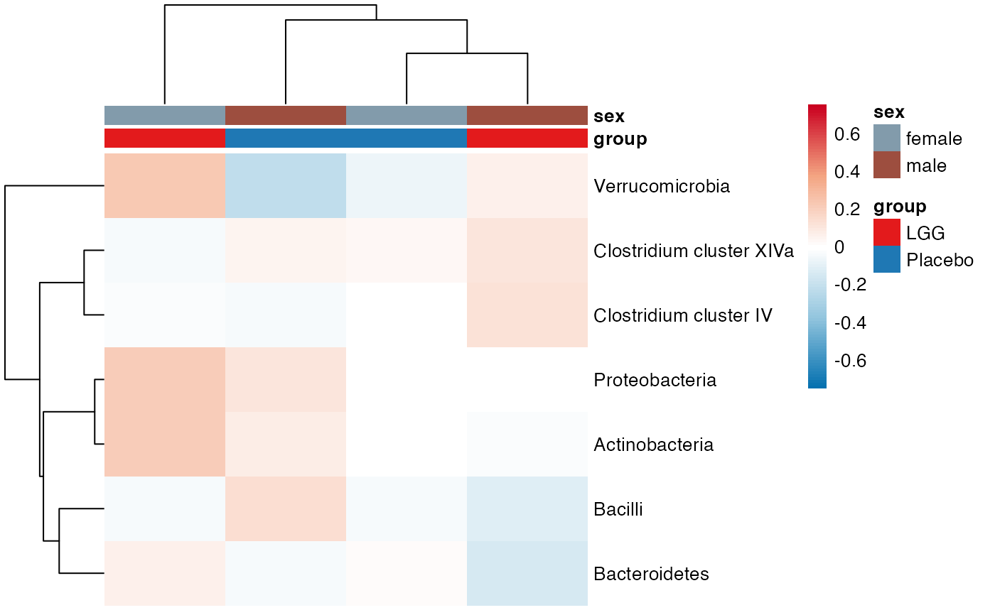 #>
#> $Family$Family$Lachnospiraceae
#>
#> $Family$Family$Lachnospiraceae
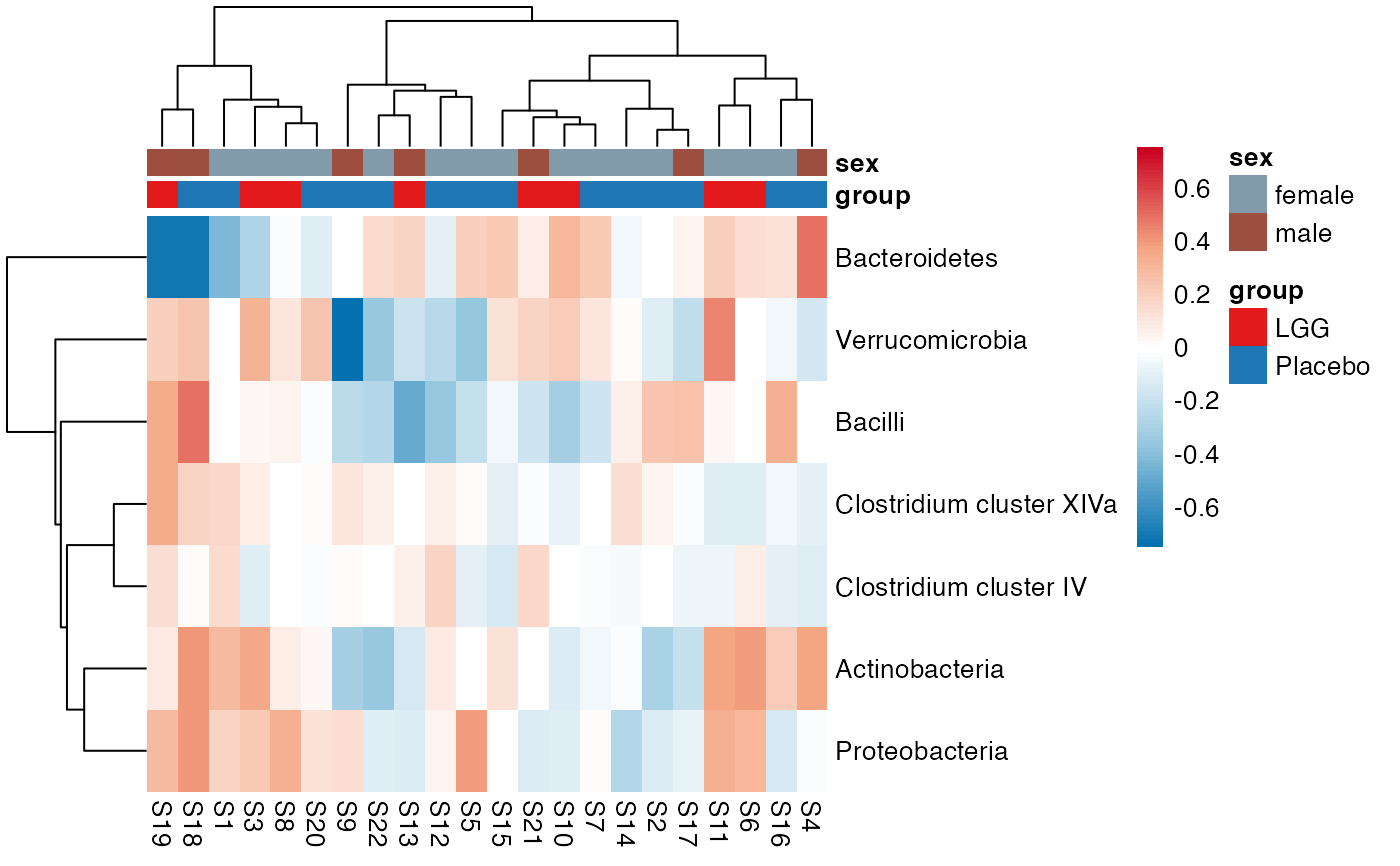 #>
#> $Family$Family$Neisseriaceae
#>
#> $Family$Family$Neisseriaceae
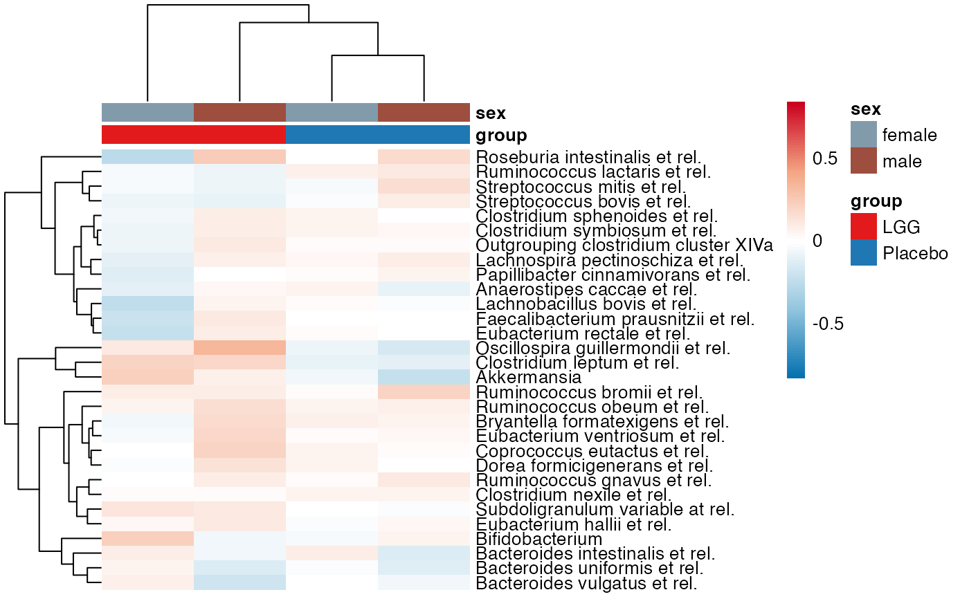 #>
#> $Family$Family$Other
#>
#> $Family$Family$Other
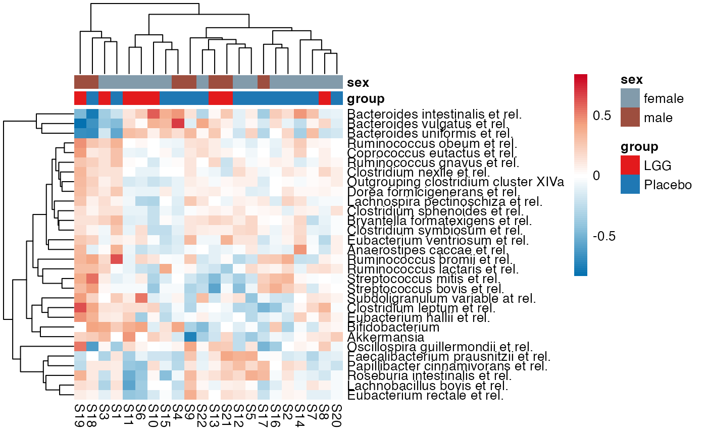 #>
#> $Family$Family$Porphyromonadaceae
#>
#> $Family$Family$Porphyromonadaceae
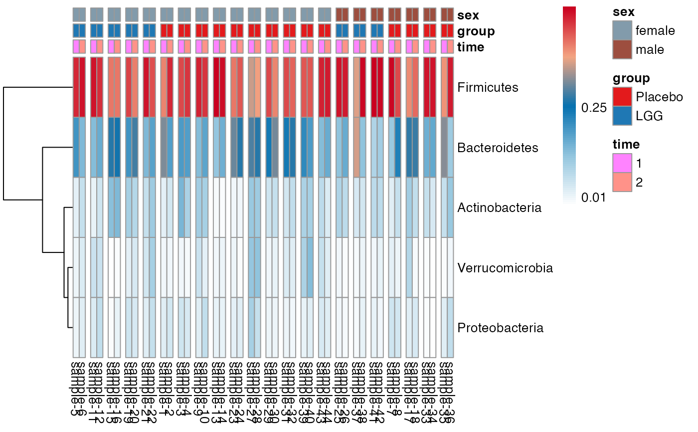 #>
#> $Family$Family$Prevotellaceae
#>
#> $Family$Family$Prevotellaceae
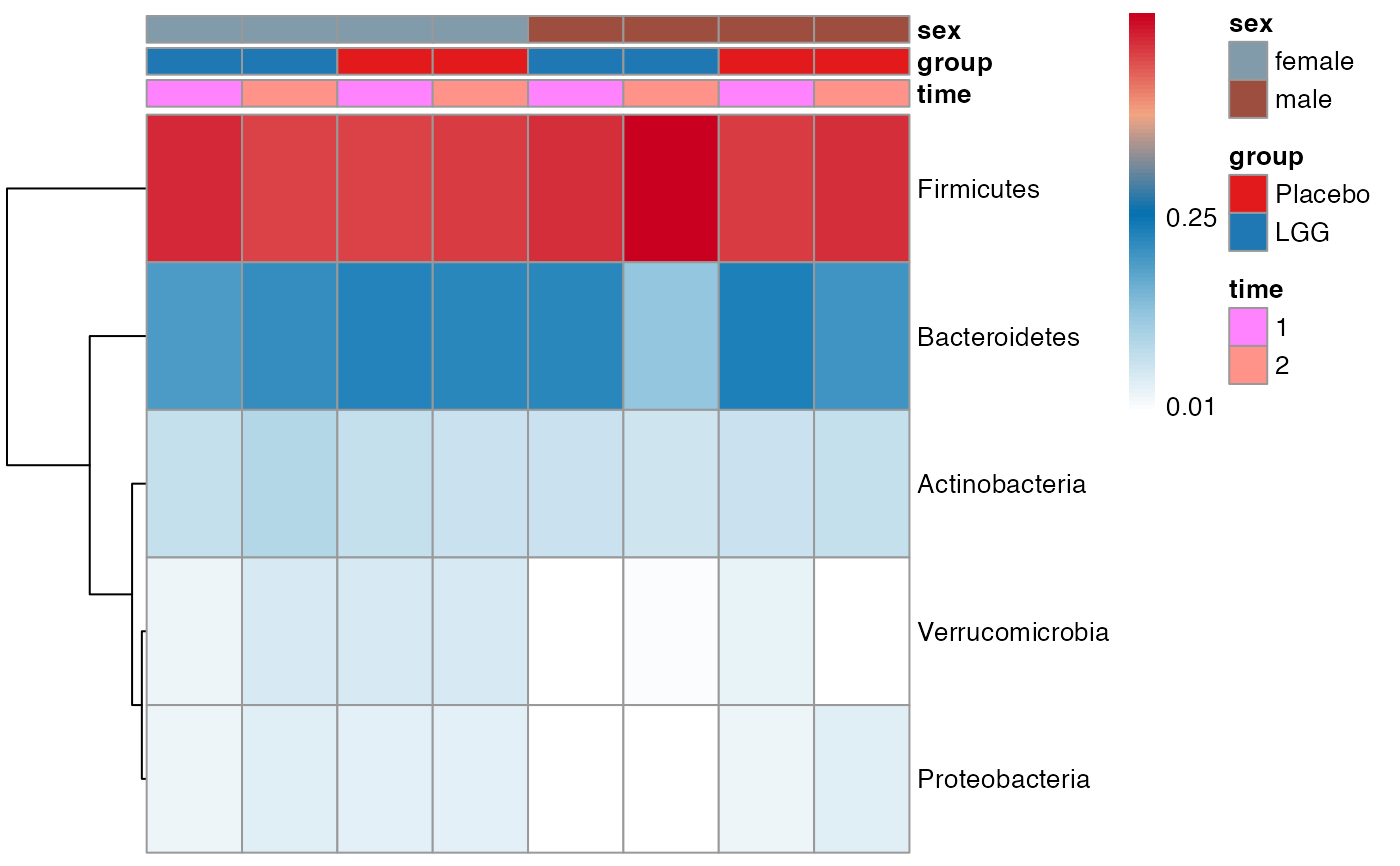 #>
#> $Family$Family$Propionibacteriaceae
#>
#> $Family$Family$Propionibacteriaceae
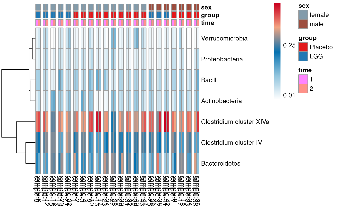 #>
#> $Family$Family$Rikenellaceae
#>
#> $Family$Family$Rikenellaceae
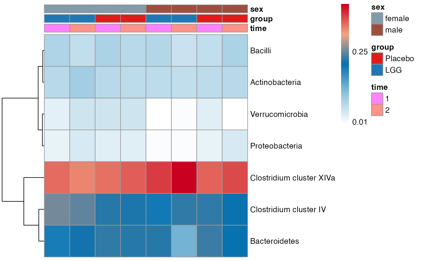 #>
#> $Family$Family$Ruminococcaceae
#>
#> $Family$Family$Ruminococcaceae
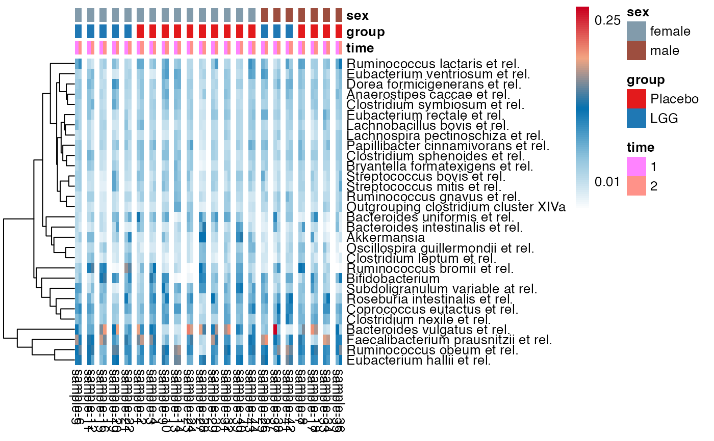 #>
#> $Family$Family$Staphylococcaceae
#>
#> $Family$Family$Staphylococcaceae
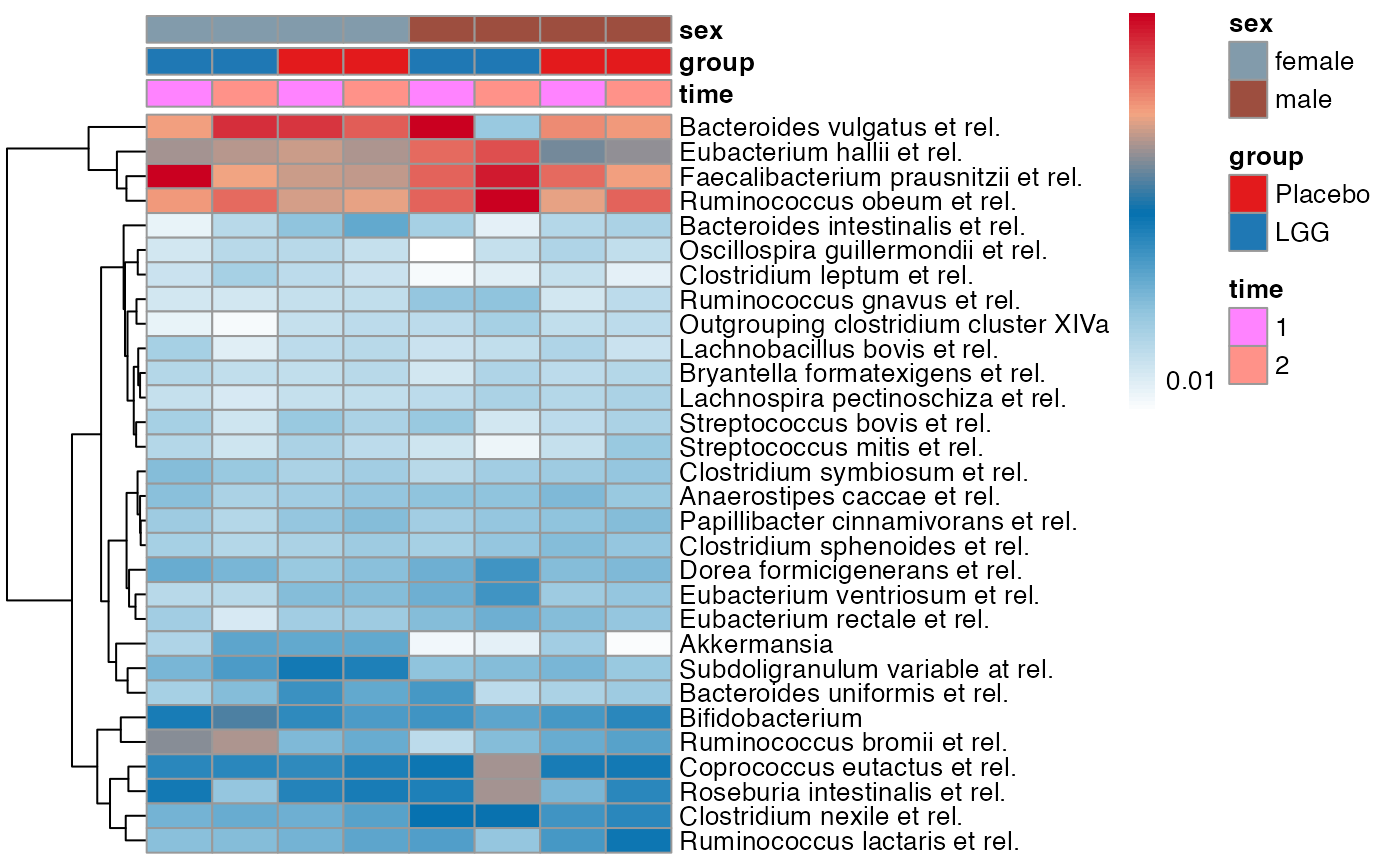 #>
#> $Family$Family$Streptococcaceae
#>
#> $Family$Family$Streptococcaceae
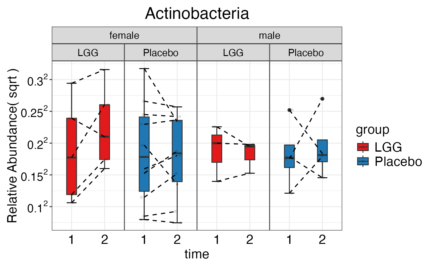 #>
#> $Family$Family$`[Tissierellaceae]`
#>
#> $Family$Family$`[Tissierellaceae]`
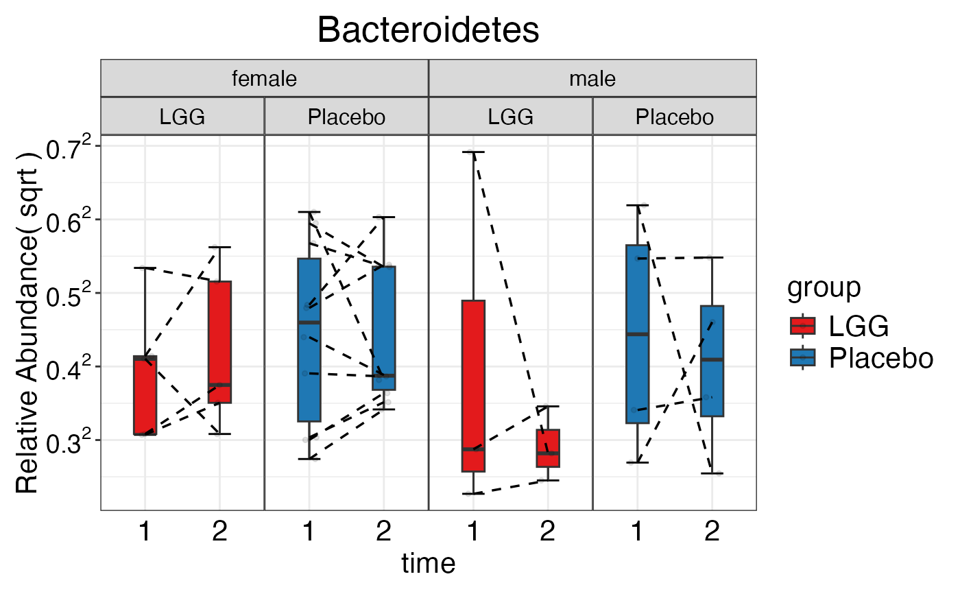 #>
#> $Family$Family$Unclassified
#>
#> $Family$Family$Unclassified
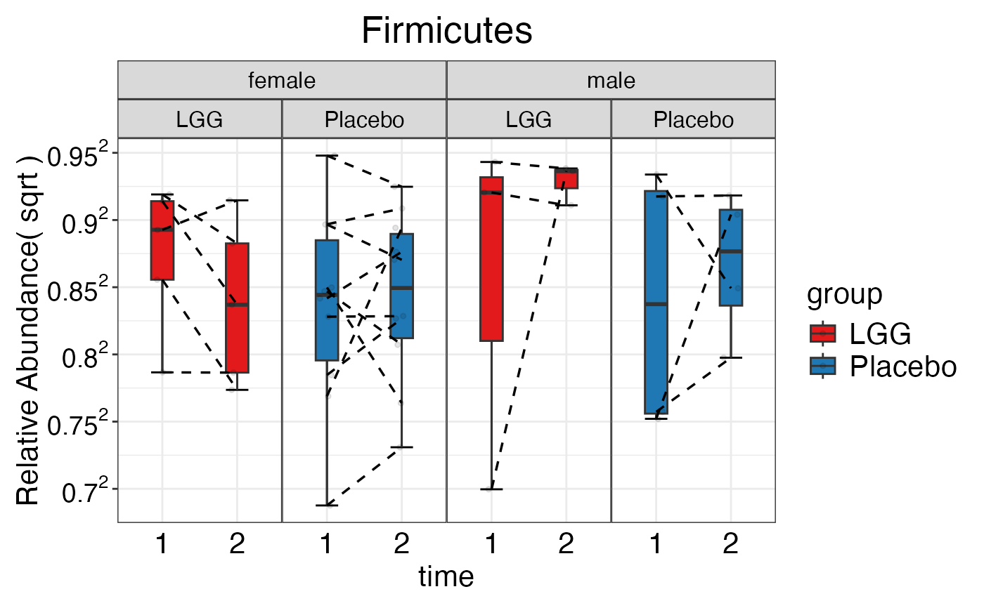 #>
#>
#>
plot_feature_diversity(
data.obj = subset_T2D.obj,
group.var = "sample_body_site",
strata.var = "subject_race",
subject.var = "subject_id",
time.var = "visit_number_num",
time.point.plot = unique(subset_T2D.obj$meta.dat$visit_number_num),
is.plot.change = FALSE,
feature.level = c("Family"),
prop.to.lump = 0.0001,
top.k.plot = NULL,
top.k.func = NULL,
renormalize = FALSE,
plot.other = TRUE,
plot.scheme = 'combined',
plot.type = "heatmap"
)
#> Validation passed.
#> Your data is in raw format ('Raw'). Normalization is crucial for further analyses. Now, 'mStat_normalize_data' function is automatically applying 'TSS' transformation.
#> Data has been successfully normalized using TSS method.
#> $Family
#> $Family$Family
#> $Family$Family$indiv
#>
#>
#>
plot_feature_diversity(
data.obj = subset_T2D.obj,
group.var = "sample_body_site",
strata.var = "subject_race",
subject.var = "subject_id",
time.var = "visit_number_num",
time.point.plot = unique(subset_T2D.obj$meta.dat$visit_number_num),
is.plot.change = FALSE,
feature.level = c("Family"),
prop.to.lump = 0.0001,
top.k.plot = NULL,
top.k.func = NULL,
renormalize = FALSE,
plot.other = TRUE,
plot.scheme = 'combined',
plot.type = "heatmap"
)
#> Validation passed.
#> Your data is in raw format ('Raw'). Normalization is crucial for further analyses. Now, 'mStat_normalize_data' function is automatically applying 'TSS' transformation.
#> Data has been successfully normalized using TSS method.
#> $Family
#> $Family$Family
#> $Family$Family$indiv
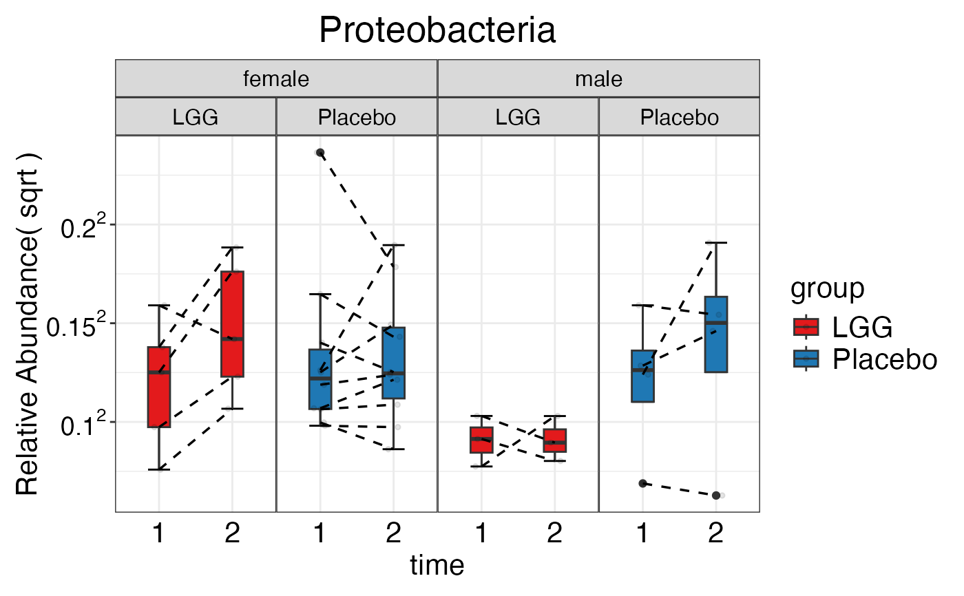 #>
#> $Family$Family$average
#>
#> $Family$Family$average
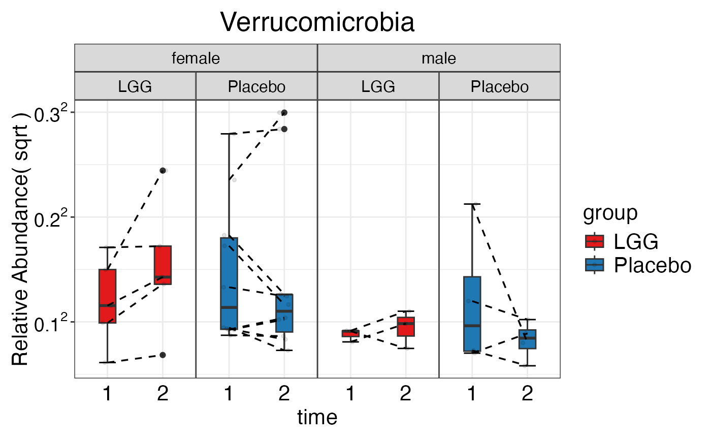 #>
#>
#>
plot_feature_diversity(
data.obj = subset_T2D.obj,
group.var = "sample_body_site",
strata.var = "subject_race",
subject.var = "subject_id",
time.var = "visit_number_num",
time.point.plot = unique(subset_T2D.obj$meta.dat$visit_number_num),
is.plot.change = TRUE,
feature.level = c("Family"),
prop.to.lump = 0.0001,
top.k.plot = NULL,
top.k.func = NULL,
renormalize = FALSE,
plot.other = TRUE,
plot.scheme = 'combined',
plot.type = "heatmap"
)
#> Validation passed.
#> Your data is in raw format ('Raw'). Normalization is crucial for further analyses. Now, 'mStat_normalize_data' function is automatically applying 'TSS' transformation.
#> Data has been successfully normalized using TSS method.
#> No columns have been removed.
#> $Family
#> $Family$Family
#>
#>
#>
plot_feature_diversity(
data.obj = subset_T2D.obj,
group.var = "sample_body_site",
strata.var = "subject_race",
subject.var = "subject_id",
time.var = "visit_number_num",
time.point.plot = unique(subset_T2D.obj$meta.dat$visit_number_num),
is.plot.change = TRUE,
feature.level = c("Family"),
prop.to.lump = 0.0001,
top.k.plot = NULL,
top.k.func = NULL,
renormalize = FALSE,
plot.other = TRUE,
plot.scheme = 'combined',
plot.type = "heatmap"
)
#> Validation passed.
#> Your data is in raw format ('Raw'). Normalization is crucial for further analyses. Now, 'mStat_normalize_data' function is automatically applying 'TSS' transformation.
#> Data has been successfully normalized using TSS method.
#> No columns have been removed.
#> $Family
#> $Family$Family
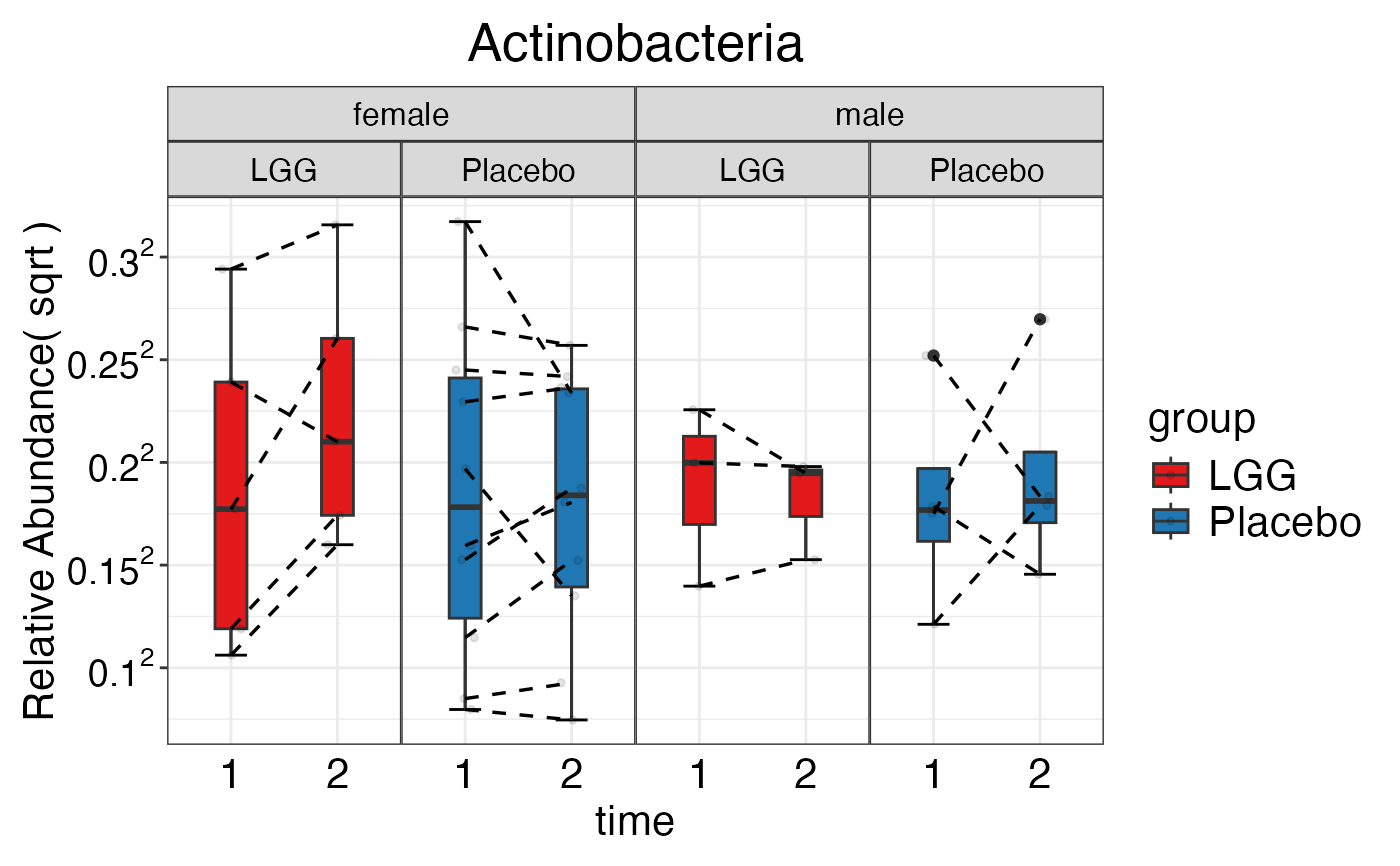 #>
#>
plot_feature_diversity(
data.obj = subset_T2D.obj,
group.var = "sample_body_site",
strata.var = "subject_race",
subject.var = "subject_id",
time.var = "visit_number_num",
time.point.plot = unique(subset_T2D.obj$meta.dat$visit_number_num),
is.plot.change = FALSE,
feature.level = c("Family"),
prop.to.lump = 0.0001,
top.k.plot = NULL,
top.k.func = NULL,
renormalize = FALSE,
plot.other = TRUE,
plot.scheme = 'combined',
plot.type = "boxplot"
)
#> Validation passed.
#> Your data is in raw format ('Raw'). Normalization is crucial for further analyses. Now, 'mStat_normalize_data' function is automatically applying 'TSS' transformation.
#> Data has been successfully normalized using TSS method.
#> $Family
#> $Family$Family
#>
#>
plot_feature_diversity(
data.obj = subset_T2D.obj,
group.var = "sample_body_site",
strata.var = "subject_race",
subject.var = "subject_id",
time.var = "visit_number_num",
time.point.plot = unique(subset_T2D.obj$meta.dat$visit_number_num),
is.plot.change = FALSE,
feature.level = c("Family"),
prop.to.lump = 0.0001,
top.k.plot = NULL,
top.k.func = NULL,
renormalize = FALSE,
plot.other = TRUE,
plot.scheme = 'combined',
plot.type = "boxplot"
)
#> Validation passed.
#> Your data is in raw format ('Raw'). Normalization is crucial for further analyses. Now, 'mStat_normalize_data' function is automatically applying 'TSS' transformation.
#> Data has been successfully normalized using TSS method.
#> $Family
#> $Family$Family
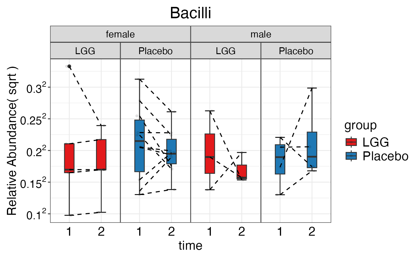 #>
#>
plot_feature_diversity(
data.obj = subset_T2D.obj,
group.var = "sample_body_site",
strata.var = "subject_race",
subject.var = "subject_id",
time.var = "visit_number_num",
time.point.plot = unique(subset_T2D.obj$meta.dat$visit_number_num),
is.plot.change = FALSE,
feature.level = c("Family"),
prop.to.lump = 0.0001,
top.k.plot = NULL,
top.k.func = NULL,
renormalize = FALSE,
plot.other = TRUE,
plot.scheme = 'individual',
plot.type = "boxplot"
)
#> Validation passed.
#> Your data is in raw format ('Raw'). Normalization is crucial for further analyses. Now, 'mStat_normalize_data' function is automatically applying 'TSS' transformation.
#> Data has been successfully normalized using TSS method.
#> $Family
#> $Family$Family
#> $Family$Family$Aerococcaceae
#>
#>
plot_feature_diversity(
data.obj = subset_T2D.obj,
group.var = "sample_body_site",
strata.var = "subject_race",
subject.var = "subject_id",
time.var = "visit_number_num",
time.point.plot = unique(subset_T2D.obj$meta.dat$visit_number_num),
is.plot.change = FALSE,
feature.level = c("Family"),
prop.to.lump = 0.0001,
top.k.plot = NULL,
top.k.func = NULL,
renormalize = FALSE,
plot.other = TRUE,
plot.scheme = 'individual',
plot.type = "boxplot"
)
#> Validation passed.
#> Your data is in raw format ('Raw'). Normalization is crucial for further analyses. Now, 'mStat_normalize_data' function is automatically applying 'TSS' transformation.
#> Data has been successfully normalized using TSS method.
#> $Family
#> $Family$Family
#> $Family$Family$Aerococcaceae
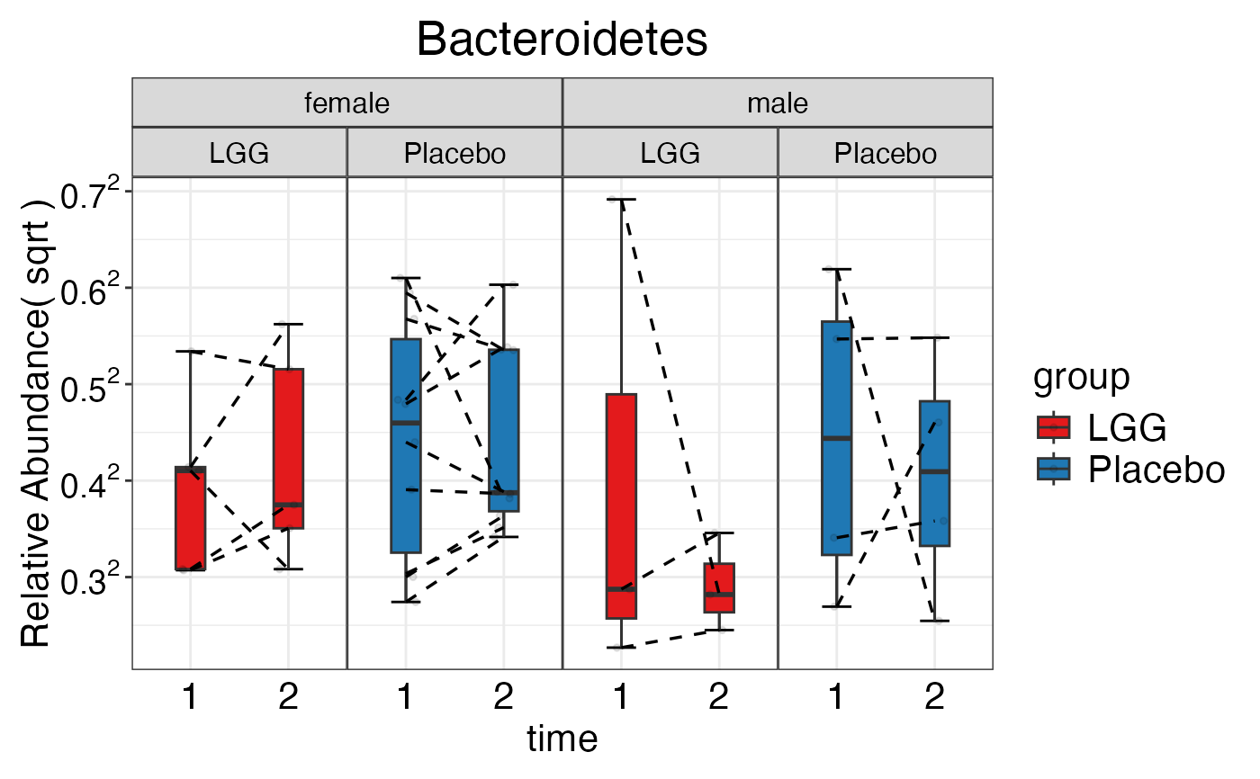 #>
#> $Family$Family$Bacteroidaceae
#>
#> $Family$Family$Bacteroidaceae
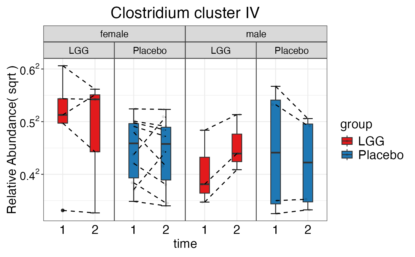 #>
#> $Family$Family$Corynebacteriaceae
#>
#> $Family$Family$Corynebacteriaceae
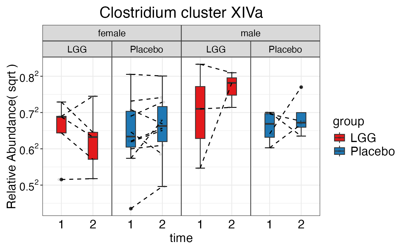 #>
#> $Family$Family$Lachnospiraceae
#>
#> $Family$Family$Lachnospiraceae
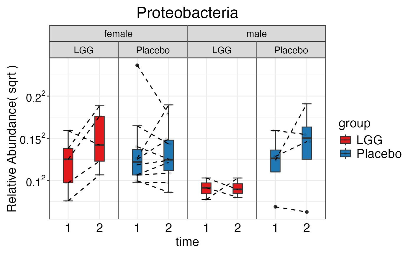 #>
#> $Family$Family$Neisseriaceae
#>
#> $Family$Family$Neisseriaceae
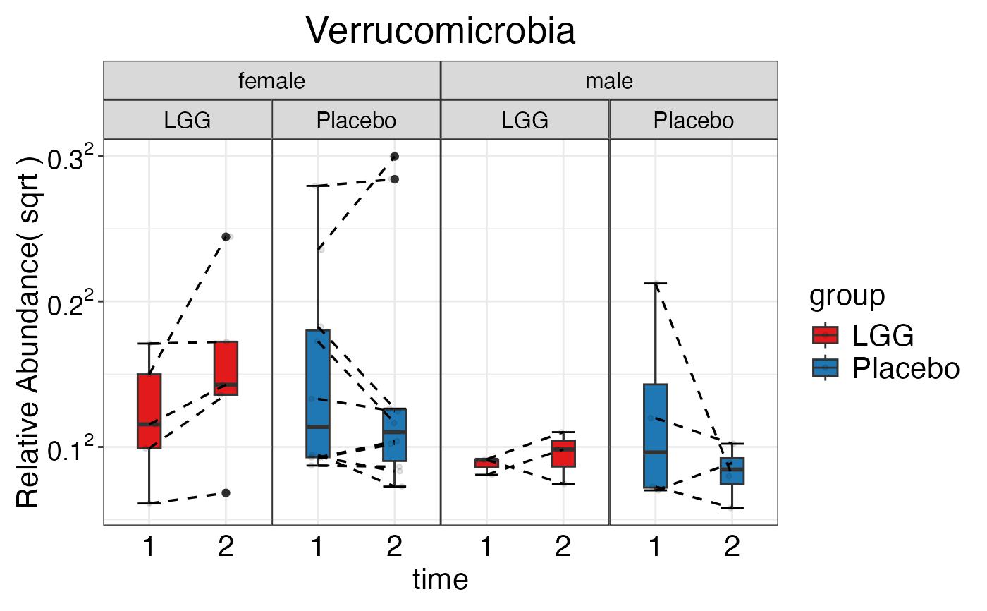 #>
#> $Family$Family$Other
#>
#> $Family$Family$Other
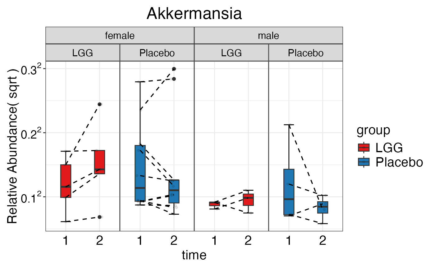 #>
#>
#>
# }
#>
#>
#>
# }