This function, part of the MicrobiomeStat package, generates various types of plots to visualize beta diversity measures in microbiome data. It supports different visualization schemes for single time point, paired time points, and longitudinal data.
Usage
plot_beta_diversity(
  dist.obj,
  pc.obj = NULL,
  meta.dat,
  measure,
  group.var = NULL,
  strata.var = NULL,
  subject.var = NULL,
  time.var = NULL,
  adj.vars = NULL,
  time.point.plot,
  is.plot.change = TRUE,
  plot.type = c("PcoA", "boxplot", "spaghettiplot"),
  ...
)
Arguments
- dist.obj
A distance matrix or object containing beta diversity measures.
- pc.obj
A matrix or data frame containing principal coordinates.
- meta.dat
A data frame containing metadata for the samples.
- measure
Character string specifying the beta diversity measure to plot.
- group.var
Character string specifying the grouping variable in meta.dat.
- strata.var
Character string specifying the stratification variable in meta.dat.
- subject.var
Character string specifying the subject variable in meta.dat.
- time.var
Character string specifying the time variable in meta.dat.
- adj.vars
Character vector specifying variables to adjust for. If specified, adjusted PCoA will be performed.
- time.point.plot
Character vector specifying time points to plot. The first point will be the reference.
- is.plot.change
Logical, whether to plot change from baseline. Only effective when there are multiple time points.
- plot.type
Character string specifying the plot type, one of c("PCoA", "boxplot", "spaghettiplot").
- ...
Additional arguments passed to the underlying plotting functions.
Details
This function provides a flexible framework for visualizing beta diversity in microbiome data. It can handle single time point, paired time points, and longitudinal data. The function offers different plot types including PCoA plots, box plots, and spaghetti plots, and can visualize changes over time.
The behavior of the function depends on the number of time points specified: - For a single time point or when time variable is not specified, only PCoA plot is available. - For two time points, both PCoA and change boxplot are available. - For more than two time points, PCoA, change boxplot, and change spaghettiplot are available.
When `is.plot.change` is TRUE and multiple time points are specified, the function will calculate changes from the baseline (first time point).
Examples
data(peerj32.obj)
dist.obj <- mStat_calculate_beta_diversity(peerj32.obj, c("BC", "Jaccard"))
#> Warning: It appears the data may not have been rarefied. Please verify.
#> Initializing distance objects...
#> Calculating Bray-Curtis dissimilarity...
#> Calculating Jaccard dissimilarity...
#> All calculations complete.
plot_beta_diversity(dist.obj = dist.obj,
meta.dat = peerj32.obj$meta.dat,
measure = c("BC", "Jaccard"),
group.var = "group",
time.var = "time",
time.point.plot = c("1"),
plot.type = "PCoA")
#> Data has been subsetted based on the provided condition.
#> Updated metadata to match the subsetted data.
#> The following samples were excluded: sample-2, sample-4, sample-6, sample-8, sample-10, sample-12, sample-14, sample-16, sample-18, sample-20, sample-22, sample-24, sample-26, sample-28, sample-30, sample-32, sample-34, sample-36, sample-38, sample-40, sample-42, sample-44
#> Data subsetting complete. Returning updated data object.
#> Calculating PC...
#> Processing BC distance...
#> Calculating MDS...
#> Processing Jaccard distance...
#> Calculating MDS...
#> Calculation complete.
#> $BC
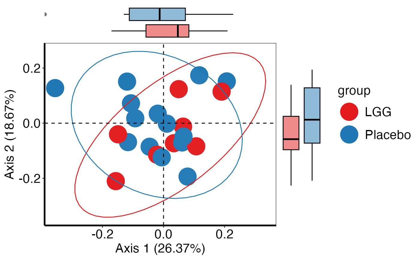 #>
#> $Jaccard
#>
#> $Jaccard
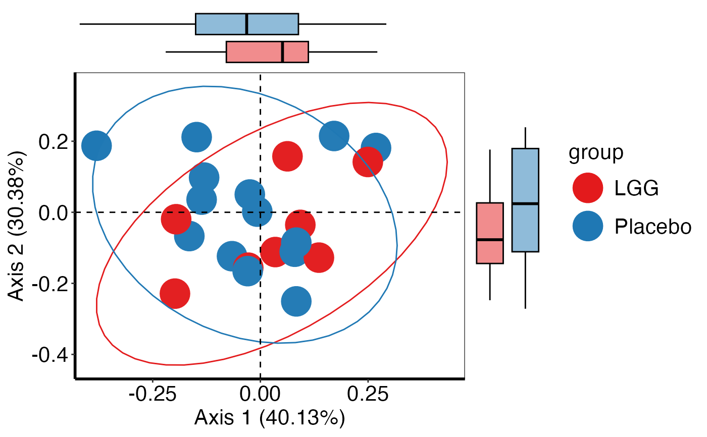 #>
plot_beta_diversity(dist.obj = dist.obj,
meta.dat = peerj32.obj$meta.dat,
measure = c("BC", "Jaccard"),
group.var = "group",
subject.var = "subject",
time.var = "time",
time.point.plot = c("1","2"),
plot.type = "PCoA",
is.plot.change = FALSE)
#> Calculating PC...
#> Processing BC distance...
#> Calculating MDS...
#> Processing Jaccard distance...
#> Calculating MDS...
#> Calculation complete.
#> Warning: Removed 22 rows containing missing values or values outside the scale range
#> (`geom_segment()`).
#> Warning: Removed 22 rows containing missing values or values outside the scale range
#> (`geom_segment()`).
#> $BC
#> Warning: Removed 22 rows containing missing values or values outside the scale range
#> (`geom_segment()`).
#>
plot_beta_diversity(dist.obj = dist.obj,
meta.dat = peerj32.obj$meta.dat,
measure = c("BC", "Jaccard"),
group.var = "group",
subject.var = "subject",
time.var = "time",
time.point.plot = c("1","2"),
plot.type = "PCoA",
is.plot.change = FALSE)
#> Calculating PC...
#> Processing BC distance...
#> Calculating MDS...
#> Processing Jaccard distance...
#> Calculating MDS...
#> Calculation complete.
#> Warning: Removed 22 rows containing missing values or values outside the scale range
#> (`geom_segment()`).
#> Warning: Removed 22 rows containing missing values or values outside the scale range
#> (`geom_segment()`).
#> $BC
#> Warning: Removed 22 rows containing missing values or values outside the scale range
#> (`geom_segment()`).
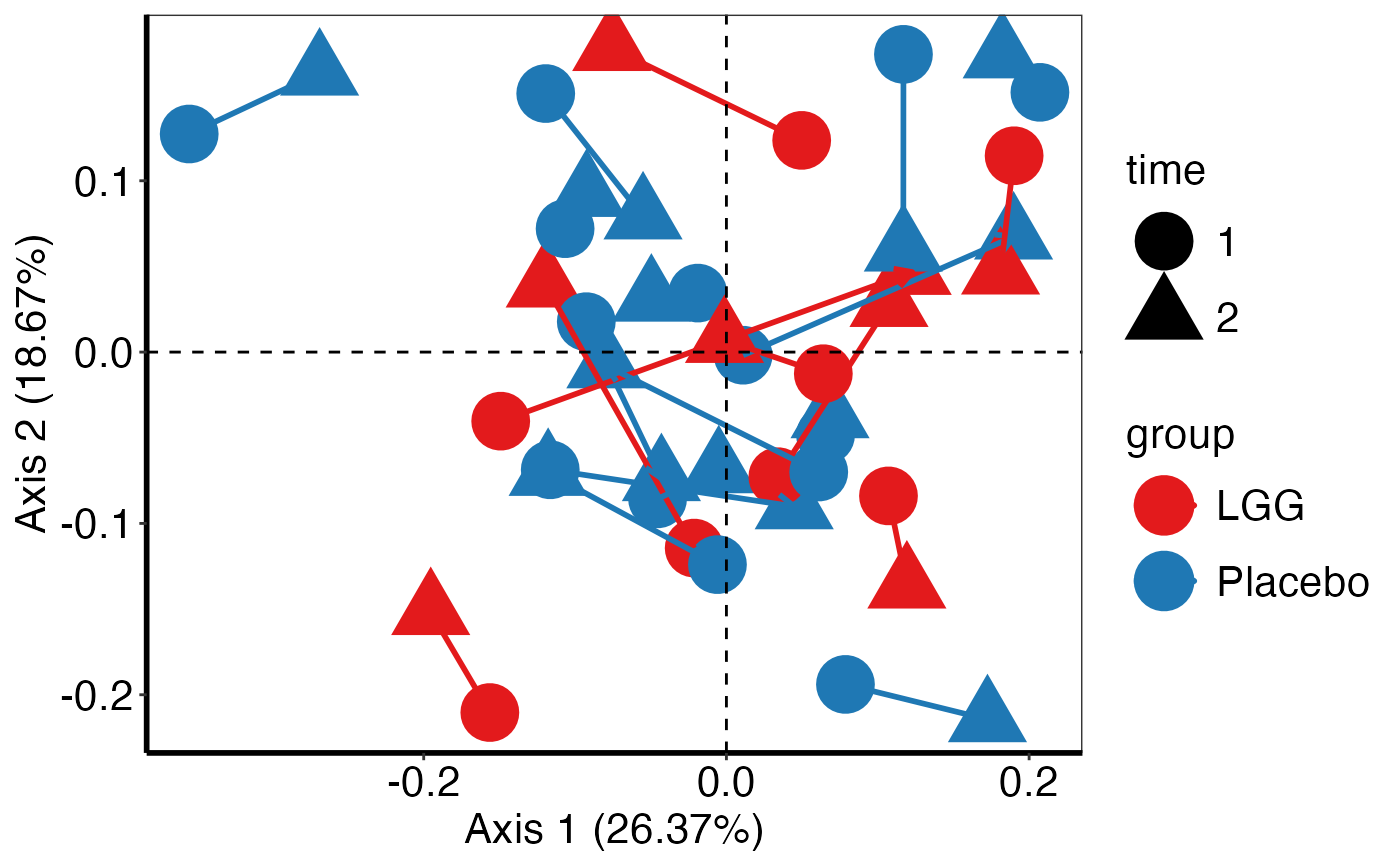 #>
#> $Jaccard
#> Warning: Removed 22 rows containing missing values or values outside the scale range
#> (`geom_segment()`).
#>
#> $Jaccard
#> Warning: Removed 22 rows containing missing values or values outside the scale range
#> (`geom_segment()`).
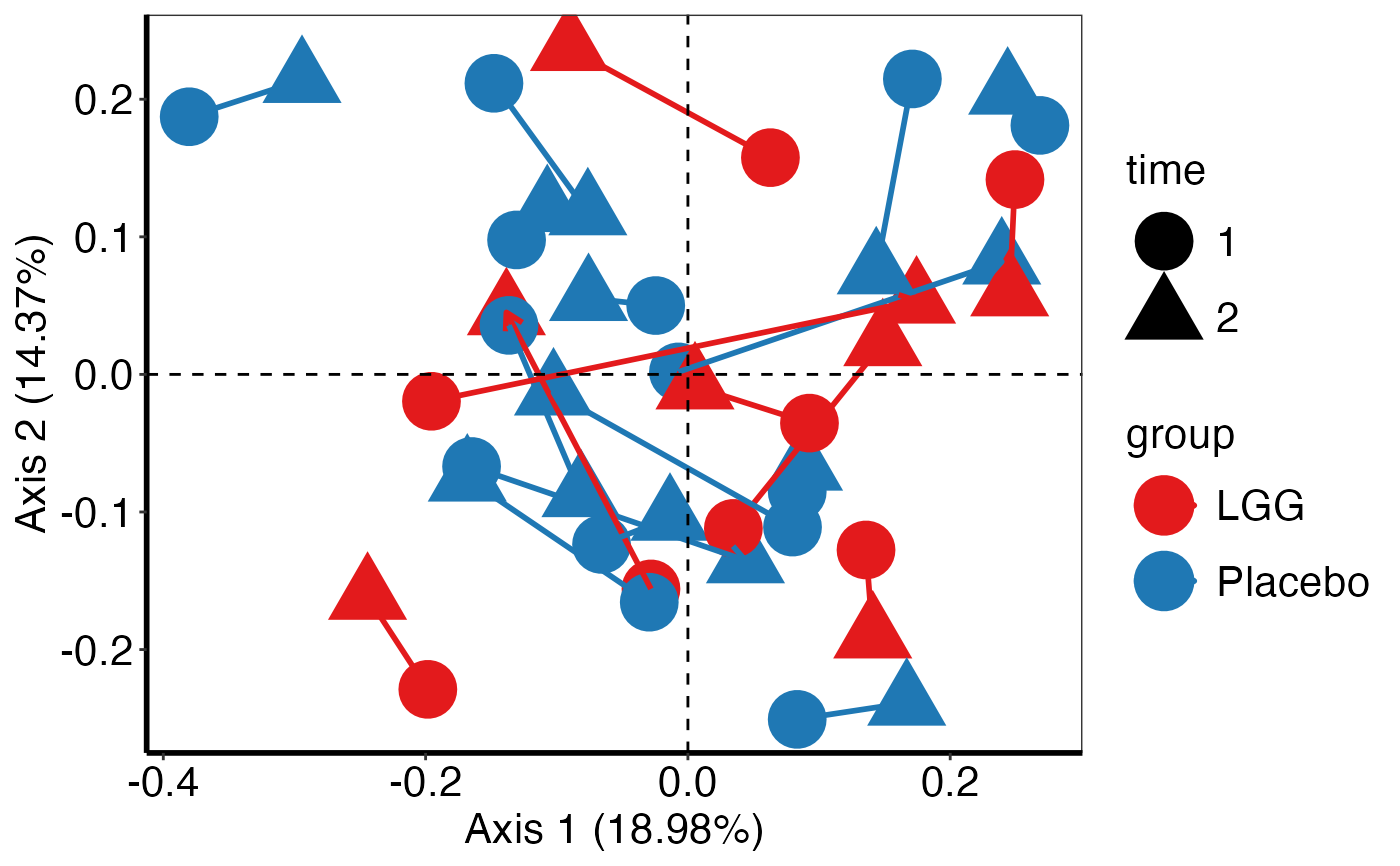 #>
plot_beta_diversity(dist.obj = dist.obj,
meta.dat = peerj32.obj$meta.dat,
measure = c("BC", "Jaccard"),
group.var = "group",
subject.var = "subject",
time.var = "time",
time.point.plot = c("1","2"),
plot.type = "boxplot",
is.plot.change = TRUE)
#> $BC
#>
plot_beta_diversity(dist.obj = dist.obj,
meta.dat = peerj32.obj$meta.dat,
measure = c("BC", "Jaccard"),
group.var = "group",
subject.var = "subject",
time.var = "time",
time.point.plot = c("1","2"),
plot.type = "boxplot",
is.plot.change = TRUE)
#> $BC
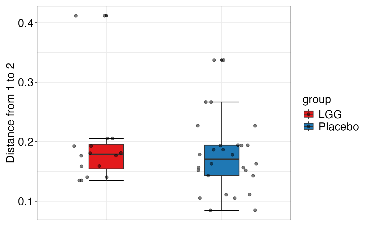 #>
#> $Jaccard
#>
#> $Jaccard
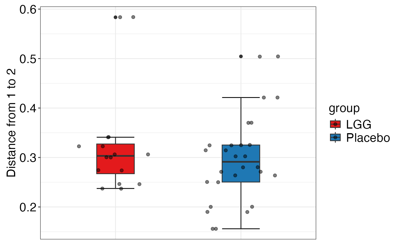 #>
data(ecam.obj)
dist.obj <- mStat_calculate_beta_diversity(ecam.obj, c("BC", "Jaccard"))
#> Warning: It appears the data may not have been rarefied. Please verify.
#> Initializing distance objects...
#> Calculating Bray-Curtis dissimilarity...
#> Calculating Jaccard dissimilarity...
#> All calculations complete.
plot_beta_diversity(dist.obj = dist.obj,
meta.dat = ecam.obj$meta.dat,
measure = c("BC", "Jaccard"),
group.var = "delivery",
subject.var = "subject.id",
time.var = "month_num",
time.point.plot = unique(ecam.obj$meta.dat$month_num),
plot.type = "boxplot",
is.plot.change = TRUE)
#> $BC
#>
data(ecam.obj)
dist.obj <- mStat_calculate_beta_diversity(ecam.obj, c("BC", "Jaccard"))
#> Warning: It appears the data may not have been rarefied. Please verify.
#> Initializing distance objects...
#> Calculating Bray-Curtis dissimilarity...
#> Calculating Jaccard dissimilarity...
#> All calculations complete.
plot_beta_diversity(dist.obj = dist.obj,
meta.dat = ecam.obj$meta.dat,
measure = c("BC", "Jaccard"),
group.var = "delivery",
subject.var = "subject.id",
time.var = "month_num",
time.point.plot = unique(ecam.obj$meta.dat$month_num),
plot.type = "boxplot",
is.plot.change = TRUE)
#> $BC
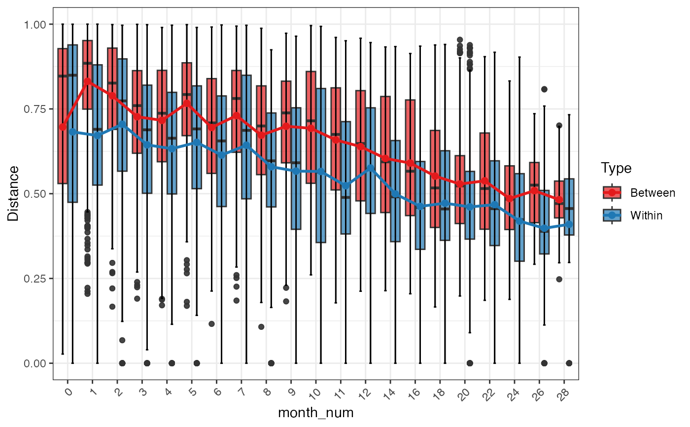 #>
#> $Jaccard
#>
#> $Jaccard
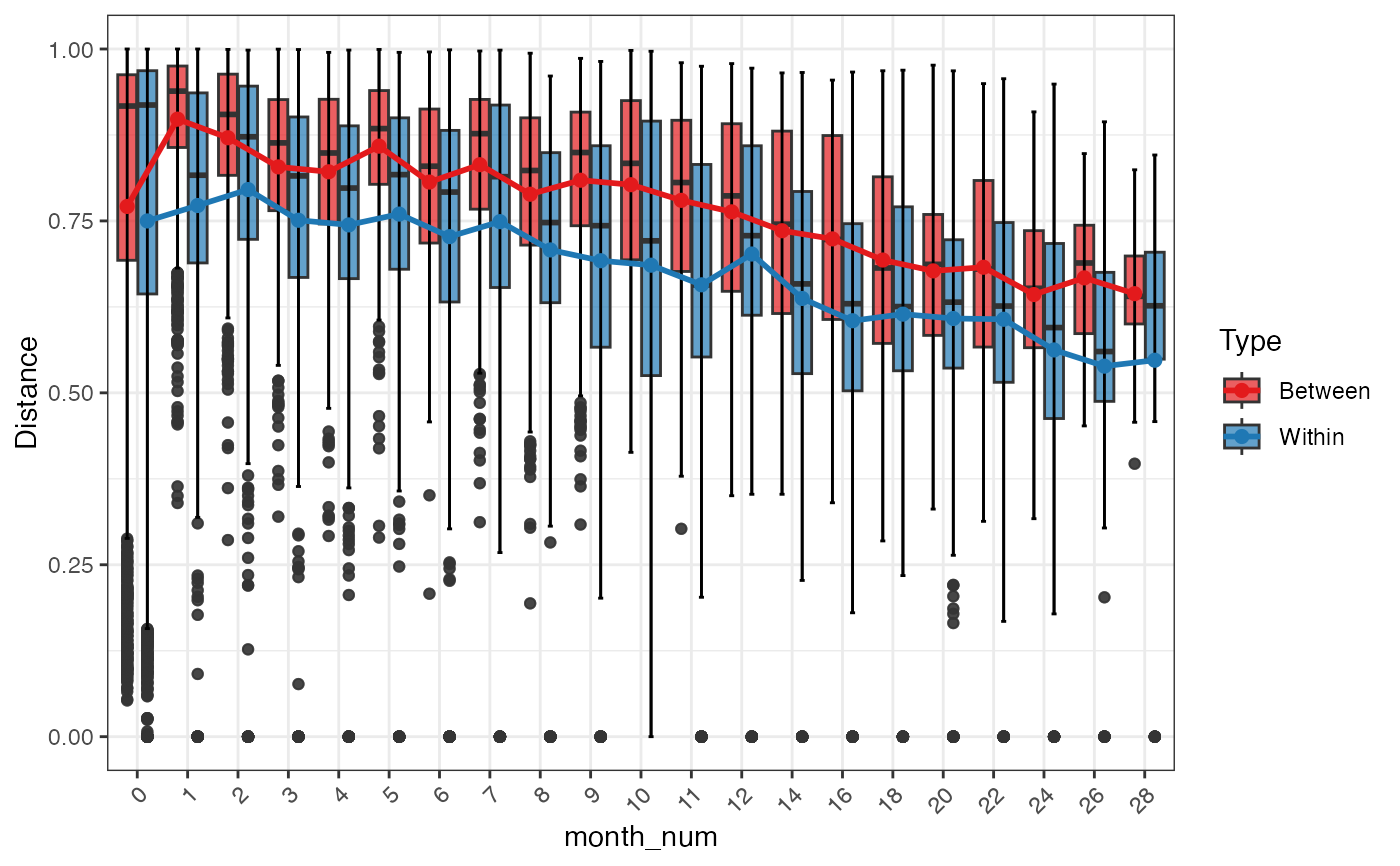 #>
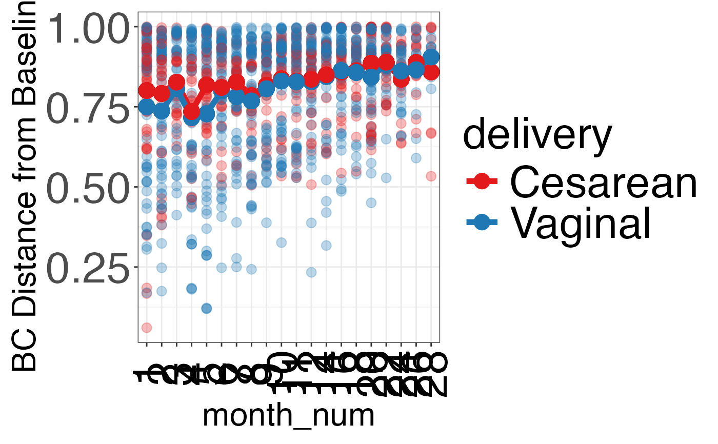
plot_beta_diversity(dist.obj = dist.obj,
meta.dat = ecam.obj$meta.dat,
measure = c("BC", "Jaccard"),
group.var = "delivery",
subject.var = "subject.id",
time.var = "month_num",
time.point.plot = unique(ecam.obj$meta.dat$month_num),
plot.type = "spaghettiplot",
is.plot.change = TRUE)
#> Note: This function requires subjects to have a baseline time point (specified by `t0.level`) to calculate the change in beta diversity. Subjects without a baseline time point will be excluded from the visualization.
#> $BC
#>
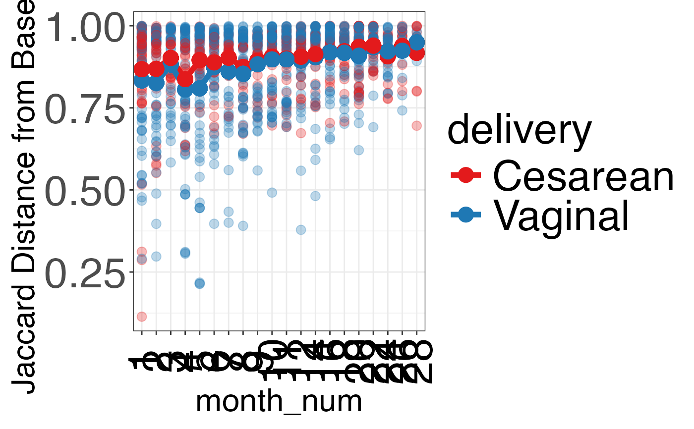
plot_beta_diversity(dist.obj = dist.obj,
meta.dat = ecam.obj$meta.dat,
measure = c("BC", "Jaccard"),
group.var = "delivery",
subject.var = "subject.id",
time.var = "month_num",
time.point.plot = unique(ecam.obj$meta.dat$month_num),
plot.type = "spaghettiplot",
is.plot.change = TRUE)
#> Note: This function requires subjects to have a baseline time point (specified by `t0.level`) to calculate the change in beta diversity. Subjects without a baseline time point will be excluded from the visualization.
#> $BC
 #>
#> $Jaccard
#>
#> $Jaccard
 #>
plot_beta_diversity(dist.obj = dist.obj,
meta.dat = ecam.obj$meta.dat,
measure = c("BC", "Jaccard"),
group.var = "delivery",
subject.var = "subject.id",
time.var = "month_num",
time.point.plot = unique(ecam.obj$meta.dat$month_num),
plot.type = "PCoA",
is.plot.change = FALSE)
#> Calculating PC...
#> Processing BC distance...
#> Calculating MDS...
#> Processing Jaccard distance...
#> Calculating MDS...
#> Calculation complete.
#> Warning: Using alpha for a discrete variable is not advised.
#> Warning: Removed 45 rows containing missing values or values outside the scale range
#> (`geom_segment()`).
#> Warning: Removed 2 rows containing missing values or values outside the scale range
#> (`geom_segment()`).
#> Warning: Using alpha for a discrete variable is not advised.
#> Warning: Removed 45 rows containing missing values or values outside the scale range
#> (`geom_segment()`).
#> Warning: Removed 2 rows containing missing values or values outside the scale range
#> (`geom_segment()`).
#> $BC
#> Warning: Using alpha for a discrete variable is not advised.
#> Warning: Removed 45 rows containing missing values or values outside the scale range
#> (`geom_segment()`).
#> Warning: Removed 2 rows containing missing values or values outside the scale range
#> (`geom_segment()`).
#>
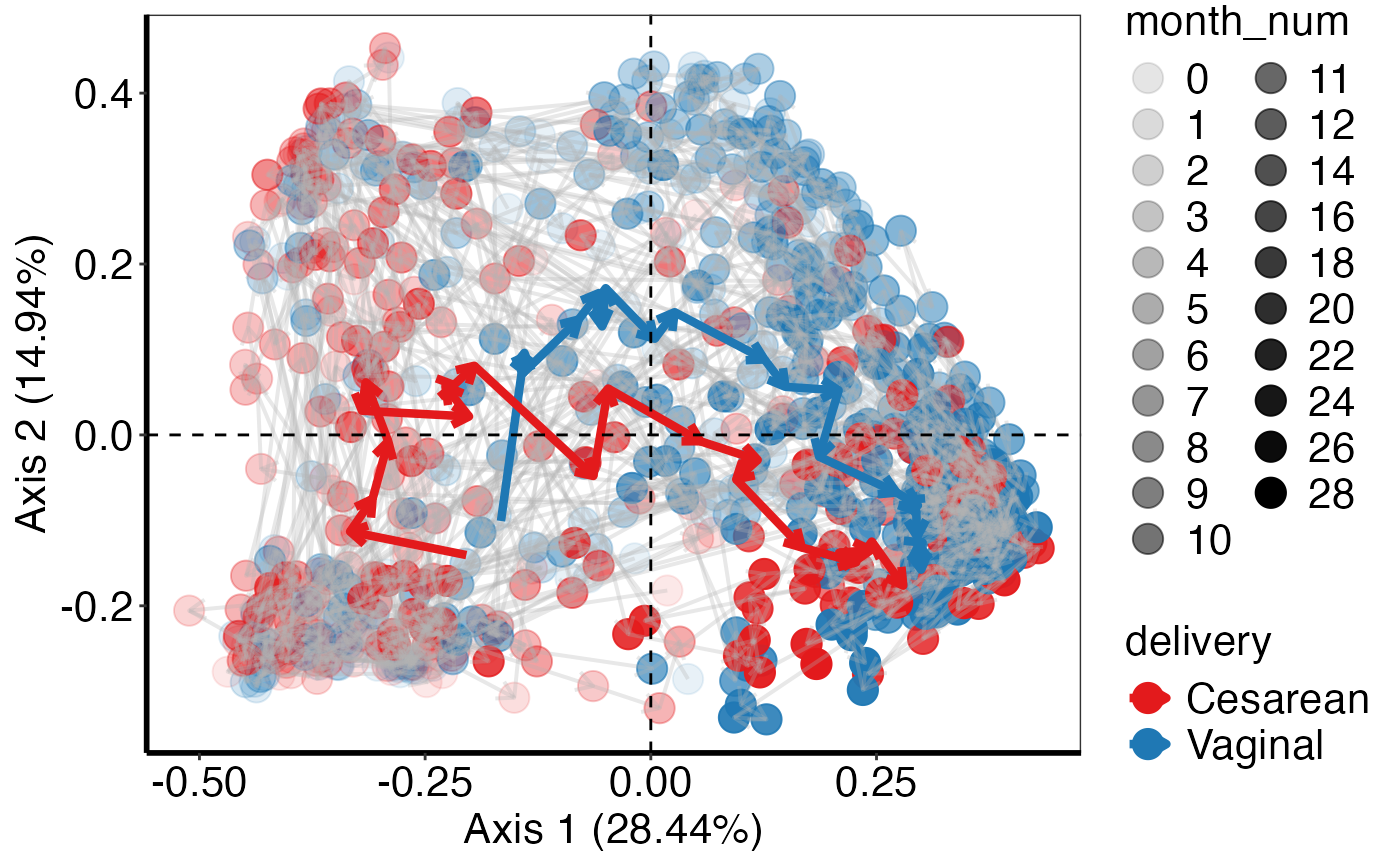
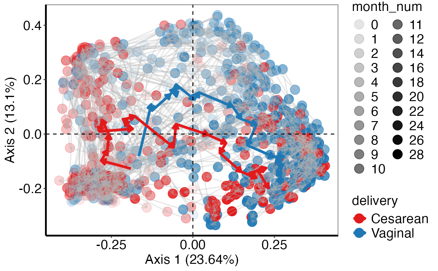
plot_beta_diversity(dist.obj = dist.obj,
meta.dat = ecam.obj$meta.dat,
measure = c("BC", "Jaccard"),
group.var = "delivery",
subject.var = "subject.id",
time.var = "month_num",
time.point.plot = unique(ecam.obj$meta.dat$month_num),
plot.type = "PCoA",
is.plot.change = FALSE)
#> Calculating PC...
#> Processing BC distance...
#> Calculating MDS...
#> Processing Jaccard distance...
#> Calculating MDS...
#> Calculation complete.
#> Warning: Using alpha for a discrete variable is not advised.
#> Warning: Removed 45 rows containing missing values or values outside the scale range
#> (`geom_segment()`).
#> Warning: Removed 2 rows containing missing values or values outside the scale range
#> (`geom_segment()`).
#> Warning: Using alpha for a discrete variable is not advised.
#> Warning: Removed 45 rows containing missing values or values outside the scale range
#> (`geom_segment()`).
#> Warning: Removed 2 rows containing missing values or values outside the scale range
#> (`geom_segment()`).
#> $BC
#> Warning: Using alpha for a discrete variable is not advised.
#> Warning: Removed 45 rows containing missing values or values outside the scale range
#> (`geom_segment()`).
#> Warning: Removed 2 rows containing missing values or values outside the scale range
#> (`geom_segment()`).
 #>
#> $Jaccard
#> Warning: Using alpha for a discrete variable is not advised.
#> Warning: Removed 45 rows containing missing values or values outside the scale range
#> (`geom_segment()`).
#> Warning: Removed 2 rows containing missing values or values outside the scale range
#> (`geom_segment()`).
#>
#> $Jaccard
#> Warning: Using alpha for a discrete variable is not advised.
#> Warning: Removed 45 rows containing missing values or values outside the scale range
#> (`geom_segment()`).
#> Warning: Removed 2 rows containing missing values or values outside the scale range
#> (`geom_segment()`).
 #>
#>
